Beware of reading signal-to-noise ratio (SNR) from power spectral density (PSD) plot
In radio communication signal analysis, for example global navigation satellite system (GNSS), a common step before analysing received signals is signal data inspection.
In radio communication signal analysis, for example global navigation satellite system (GNSS), a common step before analysing received signals is signal data inspection. This inspection step usually consists of power spectral density (PSD) and signal histogram inspections.
For PSD, either using hardware, for example spectrum analyser, or software, for example GNU radio, PSD shows power distributions with respect to frequencies, that is the bins in PSD graph. The common method to calculate PSD is Welch's method. This method is used in this post and implemented in MATLAB (including for all the figures in this post).
In this simulation, a noisy cosine waveform with frequency of $10 Hz$ is transmitted via a radio wave using carrier frequency of $950 MHz$. The noise is additive white Gaussian noise (AWGN). Commonly, after receiving this signal, we check the signal power spectral density (PSD) graph and try to estimate the signal-to-noise ratio (SNR).
Figure 1 shows the PSD of the signal. Commonly, we will guess the SNR from this PSD graph is $\pm 20 dB$. We can easily estimate this SNR by seeing the peak of the signal and the noise floor of the signal in the PSD graph. But, becareful!
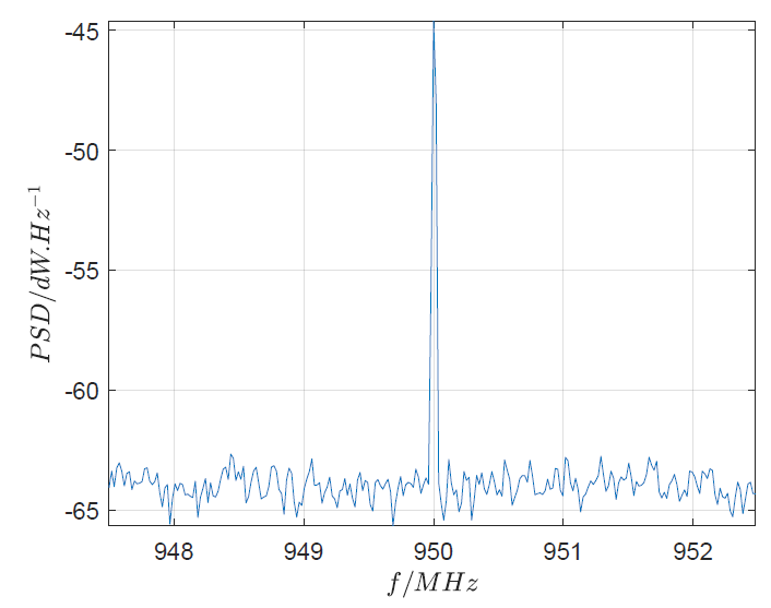
From Figure 1, we can clearly see the signal (centred at the carrier frequency of $95 MHz$), because the number of frequency bins used in figure 1 is 10000 bins. Remember that the power of the signal will be distributed to the number of frequencies, that is the number of bins in the PSD.
Figure 2 shows the PSD of the same signal with number of frequency bins of 40. In Figure 2, we cannot see the signal at all as the noise is very pronounce. Hence, our SNR reading from figure 1 is not correct.
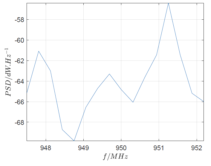
Figure 3 shows the real signal generated in the simulation. During the simulation the power of both the cosine signal and the additive white noise signal are set to be equal. Hence, the actual SNR of the noisy cosine signal is 0. In figure 3, we cannot see the cosine signal as it is buried under the noise. In figure 1, since the number of frequency bins is set high, the power of the noise is distributed to many bins resulting in low power of the noise.
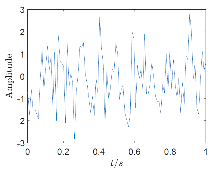
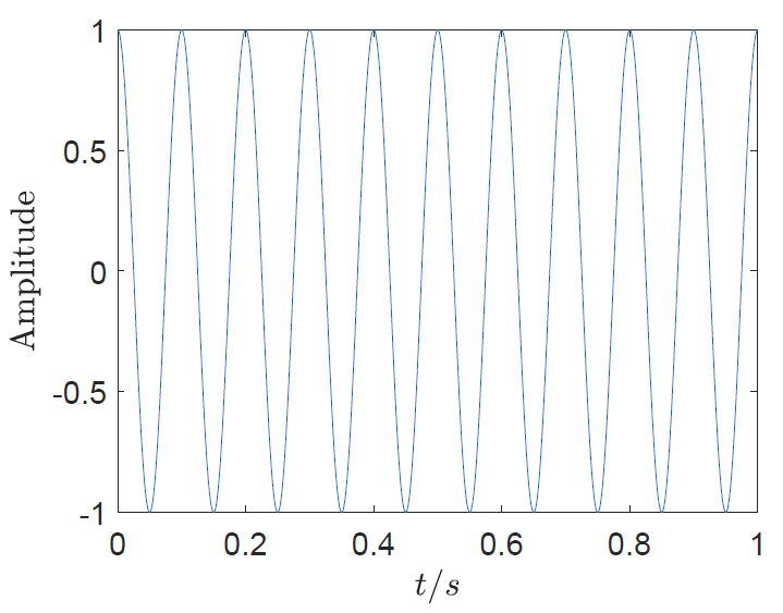
Figure 4 shows the cosine waveform when there is no noise at all. We can clearly see in this nominal cosine signal that there are ten peaks in the period of $1s$.
To conclude, beware of reading the SNR of a received signal from its PSD graph as we should take into account the number of frequency bins in the PSD as well to have a reasonable estimate of the SNR.
You may find some interesting items by shopping here.