TUTORIAL: C/C++ programming with Qt framework, OpenCV and Eigen libraries for ellipse fitting from images
This post presents how to develop and deploy an application for ellipse fitting from white blobs on images. The development is on Windows operating system. In this application, C/C++ programming language will be used along with Qt framework, OpenCV and Eigen libraries.
This post presents how to develop and deploy an application for ellipse fitting from white blobs on images. The development is on Windows operating system. In this application, C/C++ programming language will be used along with Qt framework, OpenCV and Eigen libraries.
you can get all the files in this tutorial (including the EXE file, source files and all include and LIB files) from here.
Qt framework is used to develop the graphical user interface (GUI) of the application. This framework contains Qt library to develop the GUI and Qt creator as the integrated development environment (IDE) for the editor and GUI development.
OpenCV library is used to read and show images as well as for pixel manipulation on images. Important image processing algorithms can be readily used form this library, such as image equalisation, transformation, colour transformation and thresholding.
Eigen library is used to implement matrix operations in C/C++ compiled programming language that is fast and efficient. This Eigen library try to mimic the matrix manipulation as in MATLAB programming language.
The algorithm for image processing and ellipse fitting are presented in detail. Finally, how to deploy and distribute the project source code and the compiled application will be shown at the final section.
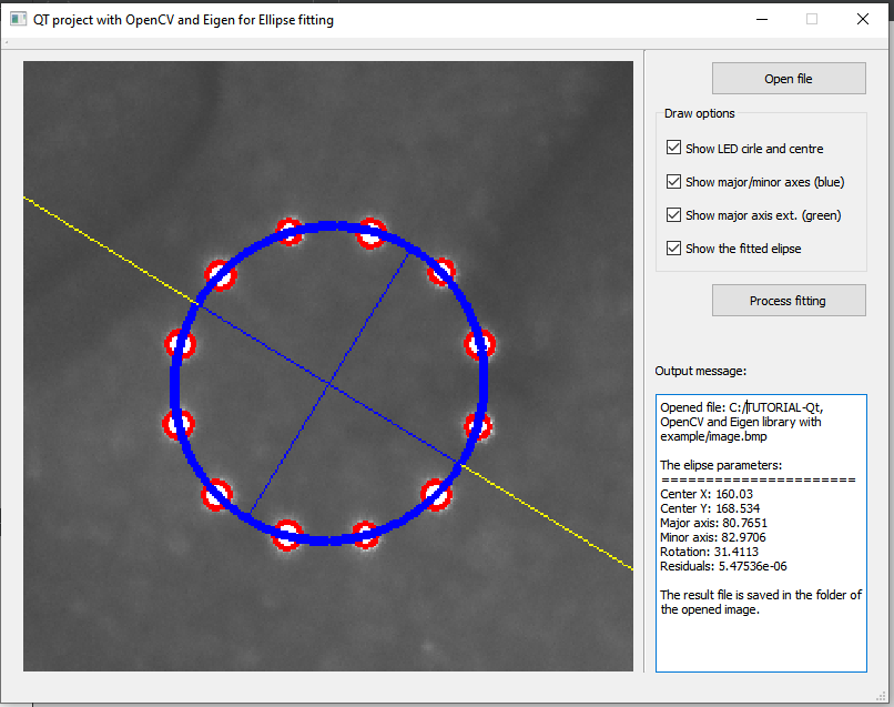
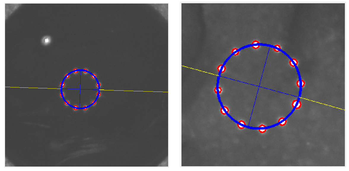
The application that we will make in this post is shown in figure 1 below. In figure 1, the application and the final ellipse fitting results are shown.
Just a reminder, in C/C++ programming language, we need to be careful when selecting the data type of a variable to avoid rounding problems in numerical data calculations.
Let us start the development!

Qt and Qt Creator: GUI design and path settings
Qt (well-known to be pronounced as “cute”) is a widget (component) framework to build a graphical user interface (GUI). The framework is mainly for C/C++ programming language. However, the framework binding for Python is also available so that the framework can be used with Python programming language.
Qt library
The Qt framework is cross-platform. This cross-platform capability makes the framework can run for multiple platforms, such as Windows, Linux, macOS and Android as well as embedded systems.
The cross-platform implementation requires no changes or very little modification of codebases using Qt. Another important advantage of cross-platform capability is that the Qt framework can run as a native application on a platform so that maximum capabilities and speed can be obtained.
The Qt framework can be downloaded from Qt download website.
Qt creator: the IDE for Qt library
Qt creator is an integrated development environment (IDE) that contains a C/C++ editor and Qt design to select and drag and drop component widgets into an application canvas.
Note that, the use of Qt creator to develop GUI based on Qt framework is not compulsory. We can use any editor or IDE that we like or familiar to use. Qt creator just an integrated IDE that make GUI design with Qt becomes easy and seamless.
Figure 2 shows the IDE of Qt creator. In figure 2, the IDE contains Qt design to design a GUI and editor to write and edit C/C++ coding.
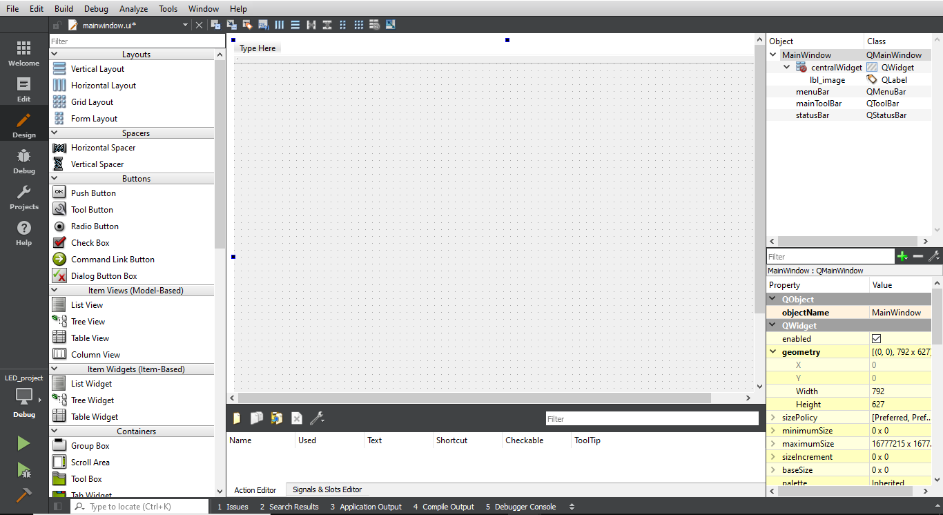

Graphical user interface (GUI) design with Qt creator integrated development environment (IDE)
The GUI development for the ellipse fitting application only requires five Qt widget components: QPushButton, QLabel, QGroupBox, QCheckBox and QTextEdit.
All of these widget components can be selected and then dragged and dropped from the Qt design section in the Qt creator to the GUI window canvas.
Figure 3 below show the GUI design and its widget components. In figure 3, the container for read images uses QLabel. The “QLabel” is set to be in black for the image container.
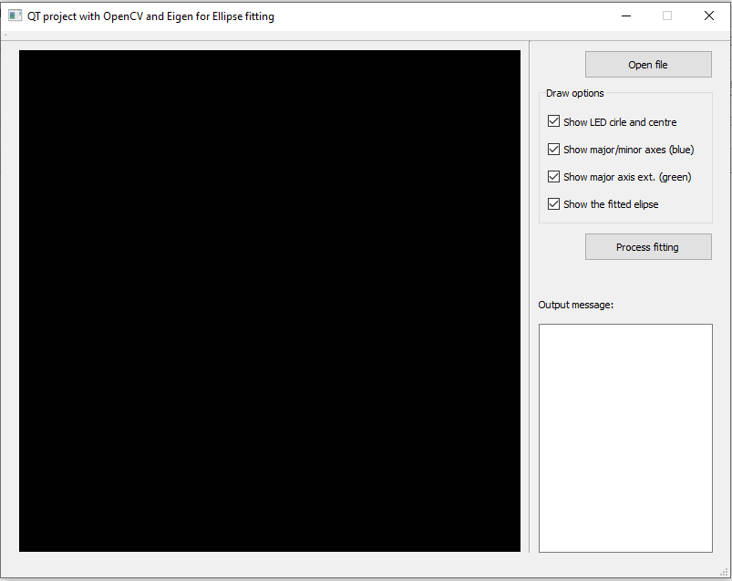
The C/C++ code to initialise the QLabel for image container to be in black is as follow:
QImage image(labelWidth, labelHeight, QImage::Format_RGB888);//Format_Indexed8 for Gray_image, Format_RGB888 for colour image
    QPixmap pixmap;
    QRgb value;
    for(int i=1;i<labelWidth;i++){
        for(int j=1;j<labelHeight;j++){
            value = qRgb(1, 1, 1);
            image.setPixel(i,j,value);
        }
    }
    pixmap = QPixmap::fromImage(image);
    ui->lbl_image->setPixmap(pixmap);
An image will be loaded to the “QLabel” (in this case is initialise as “lbl_image”) by setting the QLabel setPixmap property.
OpenCV library: read and show images, and image manipulations
OpenCV (open-source computer vision library) is a library for real-time computer vision application. OpenCV provides functions to read and show images and image manipulations as well as other computer vision-related operations.
OpenCV is a cross-platform library and is written in C/C++ language. This library can be downloaded from the OpenCV download website.
After downloading the OpenCV library from the website, we must compile the library from the source code if Windows operating system is used.
However, a compiled version of OpenCV can be found for Windows to make the installation easy. In Linux, the OpenCV download and installation can follow this guide.
Setting the OpenCV include library files
After the OpenCV installation, we must set the path for the installed OpenCV library from the Qt creator IDE.
From the “*.pro” file inside the Qt creator IDE, we can set the OpenCV include path as follow:
INCLUDEPATH += "{OpenCV_path}\OpenCV-3.1.0\opencv\build\include"
Setting the OpenCV static library for the linking process in compilation time
After setting the include path for the OpenCV library, we also need to set its static library path “*.lib” (for Windows operating system). The static library is used for the linking process in the compilation process to produce the executable (EXE) of the application.
There are two types of the static library: DEBUG and RELEASE.
DEBUG MODE is used if we want to compile the application in DEBUG mode so that we can trace and debug if there is a run-time error in the application. However, the DEBUG mode library files have larger size compared to RELEASE mode file size.
RELEASE MODE is used in case we want to compile the application for final release and for distribution. The RELEASE mode library files are much smaller than the DEBEUG files.
In the “*.pro” file, to set the static library for DEBUG is as follows:
#DEBUG
LIBS +="{OpenCV_installation_path}\lib\Debug\opencv_imgcodecs310d.lib"
LIBS +="{OpenCV_installation_path}\lib\Debug\opencv_imgproc310d.lib"
LIBS +="{OpenCV_installation_path}\lib\Debug\opencv_ml310d.lib"
LIBS +="{OpenCV_installation_path}\lib\Debug\opencv_objdetect310d.lib"
LIBS +="{OpenCV_installation_path}\lib\Debug\opencv_photo310d.lib"
LIBS +="{OpenCV_installation_path}\lib\Debug\opencv_shape310d.lib"
LIBS +="{OpenCV_installation_path}\lib\Debug\opencv_stitching310d.lib"
LIBS +="{OpenCV_installation_path}\lib\Debug\opencv_superres310d.lib"
LIBS +="{OpenCV_installation_path}\lib\Debug\opencv_ts310d.lib"
LIBS +="{OpenCV_installation_path}\lib\Debug\opencv_video310d.lib"
LIBS +="{OpenCV_installation_path}\lib\Debug\opencv_videoio310d.lib"
LIBS +="{OpenCV_installation_path}\lib\Debug\opencv_videostab310d.lib"
LIBS +="{OpenCV_installation_path}\lib\Debug\opencv_calib3d310d.lib"
LIBS +="{OpenCV_installation_path}\lib\Debug\opencv_core310d.lib"
LIBS +="{OpenCV_installation_path}\lib\Debug\opencv_features2d310d.lib"
LIBS +="{OpenCV_installation_path}\lib\Debug\opencv_flann310d.lib"
LIBS +="{OpenCV_installation_path}\lib\Debug\opencv_highgui310d.lib"
And for RELEASE is as follows:
#RELEASE
LIBS +="{OpenCV_installation_path}\lib\Release\opencv_imgcodecs310.lib"
LIBS +="{OpenCV_installation_path}\lib\Release\opencv_imgproc310.lib"
LIBS +="{OpenCV_installation_path}\lib\Release\opencv_ml310.lib"
LIBS +="{OpenCV_installation_path}\lib\Release\opencv_objdetect310.lib"
LIBS +="{OpenCV_installation_path}\lib\Release\opencv_photo310.lib"
LIBS +="{OpenCV_installation_path}\lib\Release\opencv_shape310.lib"
LIBS +="{OpenCV_installation_path}\lib\Release\opencv_stitching310.lib"
LIBS +="{OpenCV_installation_path}\lib\Release\opencv_superres310.lib"
LIBS +="{OpenCV_installation_path}\lib\Release\opencv_ts310.lib"
LIBS +="{OpenCV_installation_path}\lib\Release\opencv_video310.lib"
LIBS +="{OpenCV_installation_path}\lib\Release\opencv_videoio310.lib"
LIBS +="{OpenCV_installation_path}\lib\Release\opencv_videostab310.lib"
LIBS +="{OpenCV_installation_path}\lib\Release\opencv_calib3d310.lib"
LIBS +="{OpenCV_installation_path}\lib\Release\opencv_core310.lib"
LIBS +="{OpenCV_installation_path}\lib\Release\opencv_features2d310.lib"
LIBS +="{OpenCV_installation_path}\lib\Release\opencv_flann310.lib"
LIBS +="{OpenCV_installation_path}\lib\Release\opencv_highgui310.lib"
Including the OpenCV library in the source file
In the CPP source file, we then can include the open CV library as follows:
#include <opencv2/opencv.hpp>
#include <opencv2/highgui/highgui.hpp>
#include <opencv2/imgproc/imgproc.hpp>
#include <opencv2/imgproc/imgproc_c.h>
Eigen library: matrix operations and singular value decomposition (SVD)
Eigen library is a C++ library for the operations of linear algebra, matrix and vector. It is similar to matrix operation in MATLAB. In addition to the operations, Eigen library also provides the capability of important algebra calculations, such as geometrical transformation and numerical solver, such as singular value decomposition.
Eigen library can be downloaded from Eigen library download website.
Eigen is considered a small library. It is provided in term of C++ source and header files. We need just to include the library in the header of our C++ file and the library will be compiled together with our codes.
Setting the Eigen include library files
Since Eigen is only source file, we just need to set the path where the Eigen include libraries are. To set the include path, in the “*.pro” file (from the Qt creator IDE), we just need to add:
INCLUDEPATH += "{Eigen_file_directory}\Eigen3.2.1_library"
Including the Eigen library in the source file
To include the Eigen library in the source CPP file, we can do as follow:
#include <Eigen/Dense>
#include <Eigen/SVD>
Image processing: algorithm and C/C++ implementation with OpenCV library
In this section, the processing related to images will be presented. The processing includes image reading and presentation on “QLabel”, image blob finding and other operations.
Read and show an image on QLabel
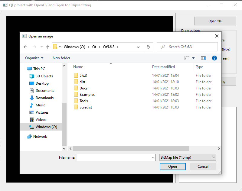
To read an image, we can use Qt library to open a file dialog so that we can search the folder and the image we want to open. The code to use the Qt file dialog is as follows:
QFileDialog *fileDlg=new QFileDialog(this);

    QString path= fileDlg->getOpenFileName(this,"Open an image","", tr("BitMap file (*.bmp);;JPEG file (*.jpg);;JPEG file (*.jpg);;PNG file (*.png)"));

    setImageFileName(path.toStdString()); //Custom function

    std::string str_val;
    str_val=path.toStdString()+".txt";

    setFileName(str_val); //custom function

    //Verify if the path has value or not
    if(path.isEmpty()){
        return;
    }
The above code will show a dialog box as shown in figure 4 below.
To show the read image on the QLabel (named “lbl_image”), the code is as follows:
QImage image;
    QPixmap pixmap;
    image = QImage((const unsigned char*)(img.data),
                                  img.cols, img.rows,
                                  img.step, QImage::Format_RGB888).rgbSwapped();
    pixmap = QPixmap::fromImage(image);

        ui->lbl_image->setPixmap(pixmap.scaled(lbl_image_width,lbl_image_height,Qt::KeepAspectRatio));
    ui->lbl_image->setAlignment(Qt::AlignCenter);

    pixmap=pixmap.scaled(lbl_image_width,lbl_image_height,Qt::KeepAspectRatio);
    pixmap_size=pixmap.size();
Finding white blobs and their centroids on an image where an ellipse fitting is applied to
In the application, an ellipse is fitted from white blobs found in an image. White blobs are areas in the image where the pixel colour is white. From these blobs, the centroid of the blobs will be obtained and used for ellipse fitting.
Before the code to find the white blob, we need to convert the BGR colour image into a binary (black and white) image. The image colour conversion can be implemented as follow:
Mat curr_image;
    img_src.copyTo(curr_image);

    //Convert to gray-scale image----------------------------------------
    Mat gray_image;
    cvtColor(curr_image, gray_image,CV_BGR2GRAY);

    //Convert to binary image--------------------------------------------
    Mat binary_image;
    threshold(gray_image, binary_image, 0, 255, CV_THRESH_BINARY | CV_THRESH_OTSU);//to make black pixel=0 and white pixel=255
After the image colour transformation colour to binary (black and white) image, the white blobs finding procedure, the calculation of the blob centroids and the filtering of unwanted blobs in the image are implemented as follow:
//finding the blobs--------------------------------------------------
    Mat binary_image_for_blobs;
    threshold(gray_image, binary_image_for_blobs, 0, 1, CV_THRESH_BINARY | CV_THRESH_OTSU);//to make black pixel=0 and white pixel=1
//return binary_image;
    vector < vector<Point2i > > blobs0;

    blobs0.clear();
    //2+ = label sign, because 0 and 1 has been used for the binary value of the image

    Mat labelled_image;
    binary_image_for_blobs.convertTo(labelled_image, CV_32SC1); //it has to be able to store integer up to a large value, because the number of blobs can be very large

    int label_count = 2; // starts from 2 because 0 and 1 have been used already

    for(int y=0; y < labelled_image.rows; y++) {
        int *row = (int*)labelled_image.ptr(y);
        for(int x=0; x < labelled_image.cols; x++) {
            if(row[x] != 1 && row[x] != 0) {//if the pixel has been labelled, continue (the binary pixel are 0 or 1)
                continue;
            }

            //Labelling process ----------------------------------------------------
            Rect rect;
            floodFill(labelled_image, Point(x,y), label_count, &rect, 0, 0, 4); //or 8

            vector <Point2i> blob;

            for(int i=rect.y; i < (rect.y+rect.height); i++) {
                int *row2 = (int*)labelled_image.ptr(i);
                for(int j=rect.x; j < (rect.x+rect.width); j++) {
                    if(row2[j] != label_count) {
                        continue;
                    }

                    blob.push_back(Point2i(j,i));
                }
            }
The procedure to filter of outlier blobs (blobs that are very far from the other blobs and too big or too small) in the image are implemented as follow:
            //filter out unwanted blob: check the blob area AND the width - height ration
            float width_height_ratio=1.0;

            //find the width_heigth ratio
            int maxX, minX, maxY, minY;
            maxX=-99999;
            minX=99999;
            maxY=-9999;
            minY=9999;
            for(int k=0;k<blob.size();k++){
                Point2i pt=blob[k];
                if(maxX<pt.x){
                    maxX=pt.x;
                }
                if(maxY<pt.y){
                    maxY=pt.y;
                }
                if(minX>pt.x){
                    minX=pt.x;
                }
                if(minY>pt.y){
                    minY=pt.y;
                }
            }

            float width=(maxX-minX)/2;
            float height=(maxY-minY)/2;
            width_height_ratio=width/height;

            if((blob.size()>=MIN_BLOB_AREA && blob.size()<MAX_BLOB_AREA) && (width_height_ratio>=0.3 &&width_height_ratio<=1.8)){
            ){
                if(minX>5 && maxX<labelled_image.cols-5 && minY>5 && maxY<labelled_image.rows-5){//Remove blobs near the edge
                    blobs0.push_back(blob);
                }
                else{//the blob is excluded due to too close to the edge
                    blobs_on_edge++;
                }
            }

            label_count++;
        }
    }

//Filtering the unwanted blob ----------------------------------------------------------------------
    vector<Point2f> centre_BLOB;
    for(int i=0;i<blobs0.size();i++){
        vector <Point2i> blob=blobs0[i];
        int maxX, minX, maxY, minY;
        maxX=-99999;
        minX=99999;
        maxY=-9999;
        minY=9999;
        for(int j=0;j<blob.size();j++){
            Point2i pt=blob[j];
            if(maxX<pt.x){
                maxX=pt.x;
            }
            if(maxY<pt.y){
                maxY=pt.y;
            }
            if(minX>pt.x){
                minX=pt.x;
            }
            if(minY>pt.y){
                minY=pt.y;
            }
        }

        float centreX=(minX+maxX)/2;
        float centreY=(minY+maxY)/2;

        centre_BLOB.push_back(Point2f(centreX,centreY));
    }
The blob filtering process is to detect outlier blob and remove form the set of the blobs used for the ellipse fitting. Figure 5 below shows an example of detecting outlier blobs.
The calculation of the blob centroids is as follows:
float temp_centroid_x=0;
    float temp_centroid_y=0;
    float temp_sum1=0,temp_sum2=0;
    for(int i=0;i<blobs0.size();i++){
        Point2f curr_centre_LED =centre_BLOB[i];
        temp_sum1=temp_sum1+curr_centre_BLOB.x;
        temp_sum2=temp_sum2+curr_centre_BLOB.y;
    }
    temp_centroid_x=temp_sum1/blobs0.size();
    temp_centroid_y=temp_sum2/blobs0.size();

    //inserting the valid blob to blobs
    vector < vector<Point2i > > blobs;
    blobs.clear();

    for(int i=0;i<blobs0.size();i++){
        float dist=0.0;
        Point2f curr_centre_BLOB =centre_BLOB[i];
        float temp_val=(float)pow(temp_centroid_x-curr_centre_BLOB.x,2)+(float)pow(temp_centroid_y-curr_centre_BLOB.y,2);
        dist=(float)pow(temp_val,0.5);
        if(dist > SMALLEST_DISTANCE && dist<LARGEST_DISTANCE){
            blobs.push_back(blobs0[i]);
        }

    }

    if((blobs.size()+blobs_on_edge)>=10){
        //if BLOB found < 10 --> recalculate the centre with the given blobs
        //and re-select the blob from the blobs0
        flag_BLOB_found=1;
    }
    else{
        flag_BLOB_found=0;
    }
Plot a fitted ellipse on the image shown in the QLabel
After fitting an ellipse (the ellipse fitting will be explained in the next section), from the fitted ellipse parameters (the x and y coordinates of the centre point, the major and minor axes and the tilt angle), we can draw the ellipse on the image shown in the lbl_image (QLabel).
The code to draw the ellipse is as follows:
Mat plotted_img;
    img_src.copyTo(plotted_img);

    const float phi=3.14;
    float rotAxis_in_rad=rotAxis*phi/180;

    int num_point=500;
    float step_size=2*phi/num_point;
    float t=0.0; //already in radian
    for(int i=0;i<num_point;i++){
        float x=0,y=0;

        x=cx+(cos(rotAxis_in_rad)*majorAxis*cos(t)-sin(rotAxis_in_rad)*minorAxis*sin(t));
        y=cy+(sin(rotAxis_in_rad)*majorAxis*cos(t)+cos(rotAxis_in_rad)*minorAxis*sin(t));

        t=t+step_size;

        Scalar color=Scalar( 255, 0, 0);//blue: BGR format
        Point centre_point_int;
        centre_point_int.x=(int)round(x);
        centre_point_int.y=(int)round(y);
        circle(plotted_img,centre_point_int, 0, color, 4, 8, 0 );
    }
Plot the major and minor axes of a fitted ellipse on the image shown in the QLabel
After drawing the fitted ellipse, we then draw the major and minor axis of the ellipse. The codes to draw the major and minor axes are as follows:
img_src.copyTo(plotted_img);

    Scalar color=Scalar( 255, 0, 0);//blue: BGR format
    float x=0,y=0;
    Point2f start,end;

    const float PHI=3.14;
    float rotAxis_in_rad=rotAxis*PHI/180;
    float phi=0;

    //Major axis
    //at phi =0
    phi=0*PHI/180;
    x=cx+(cos(rotAxis_in_rad)*majorAxis*cos(phi)-sin(rotAxis_in_rad)*minorAxis*sin(phi));
    y=cy+(sin(rotAxis_in_rad)*majorAxis*cos(phi)+cos(rotAxis_in_rad)*minorAxis*sin(phi));
    start.x=(int)round(x);
    start.y=(int)round(y);
    //at phi=180
    phi=180*PHI/180;
    x=cx+(cos(rotAxis_in_rad)*majorAxis*cos(phi)-sin(rotAxis_in_rad)*minorAxis*sin(phi));
    y=cy+(sin(rotAxis_in_rad)*majorAxis*cos(phi)+cos(rotAxis_in_rad)*minorAxis*sin(phi));
    end.x=(int)round(x);
    end.y=(int)round(y);
    line(plotted_img,start,end, color, 1,LINE_8);

    //Minor axis
    //at phi =90
    phi=90*PHI/180;
    x=cx+(cos(rotAxis_in_rad)*majorAxis*cos(phi)-sin(rotAxis_in_rad)*minorAxis*sin(phi));
    y=cy+(sin(rotAxis_in_rad)*majorAxis*cos(phi)+cos(rotAxis_in_rad)*minorAxis*sin(phi));
    start.x=(int)round(x);
    start.y=(int)round(y);
    //at phi=270
    phi=270*PHI/180;
    x=cx+(cos(rotAxis_in_rad)*majorAxis*cos(phi)-sin(rotAxis_in_rad)*minorAxis*sin(phi));
    y=cy+(sin(rotAxis_in_rad)*majorAxis*cos(phi)+cos(rotAxis_in_rad)*minorAxis*sin(phi));
    end.x=(int)round(x);
    end.y=(int)round(y);
    line(plotted_img,start,end, color, 1,LINE_8);
Plot the extension of the major and minor axes of a fitted ellipse on the image shown in the QLabel
In addition to the major and minor axes of the fitted ellipse, we then now draw the extension of the major and minor axes.
Note that to draw the extension, we need to divide the drawing process depending on where the fitted ellipse is located inside the image.
The codes to draw the extension axes are as follow:
Mat plotted_img;
    img_src.copyTo(plotted_img);

    int maxX=plotted_img.cols;
    int maxY=plotted_img.rows;

    Scalar color=Scalar( 0, 255, 255);//yellow: BGR format
    float xa=0,ya=0, xb=0,yb=0, x1=0, y1=0;
    Point2f start1,end1,start2,end2;

    const float PHI=3.14;
    float rotAxis_in_rad=rotAxis*PHI/180;
    float phi=0;

    float gradient1=0.0,gradient2=0.0;

    //Major axis 1
    //at phi =0
    phi=0*PHI/180;
    xa=cx+(cos(rotAxis_in_rad)*majorAxis*cos(phi)-sin(rotAxis_in_rad)*minorAxis*sin(phi));
    ya=cy+(sin(rotAxis_in_rad)*majorAxis*cos(phi)+cos(rotAxis_in_rad)*minorAxis*sin(phi));
    start1.x=(int)round(xa);
    start1.y=(int)round(ya);

    //Major axis 2
    //at phi=180
    phi=180*PHI/180;
    xb=cx+(cos(rotAxis_in_rad)*majorAxis*cos(phi)-sin(rotAxis_in_rad)*minorAxis*sin(phi));
    yb=cy+(sin(rotAxis_in_rad)*majorAxis*cos(phi)+cos(rotAxis_in_rad)*minorAxis*sin(phi));
    start2.x=(int)round(xb);
    start2.y=(int)round(yb);


    if(start1.y<start2.y){
        if(xa<maxX/2){
            //line1
            gradient1 = (cy-ya)/(cx-xa); //y-y1=m(x-x1)
            x1=0;
            y1=ya-(gradient1*(xa-x1));
            if(y1<0){
                y1=0;
                x1=((ya-y1)-gradient1*xa)/(-gradient1);
            }

            end1.x=(int)round(x1);
            end1.y=(int)round(y1);

            //line2
            gradient2 = (cy-yb)/(cx-xb); //y-y1=m(x-x1)

            x1=maxX;
            y1=yb-(gradient2*(xb-x1));
            if(y1>=maxY){
                y1=maxY;
                x1=((yb-y1)-gradient2*xb)/(-gradient2);
            }

            end2.x=(int)round(x1);
            end2.y=(int)round(y1);
        }
        else{
            //line1
            gradient1 = (cy-ya)/(cx-xa); //y-y1=m(x-x1)
            x1=maxX;
            y1=ya-(gradient1*(xa-x1));
            if(y1<0){
                y1=0;
                x1=((ya-y1)-gradient1*xa)/(-gradient1);
            }

            end1.x=(int)round(x1);
            end1.y=(int)round(y1);

            //line2
            gradient2 = (cy-yb)/(cx-xb); //y-y1=m(x-x1)

            x1=0;
            y1=yb-(gradient2*(xb-x1));
            if(y1>=maxY){
                y1=maxY;
                x1=((yb-y1)-gradient2*xb)/(-gradient2);
            }

            end2.x=(int)round(x1);
            end2.y=(int)round(y1);
        }

    }
    else{
        if(xa>=maxX/2){
            //line1
            gradient1 = (cy-ya)/(cx-xa); //y-y1=m(x-x1)
            x1=maxX;
            y1=ya-(gradient1*(xa-x1));
            if(y1>maxY){
                y1=maxY;
                x1=((ya-y1)-gradient1*xa)/(-gradient1);
            }

            end1.x=(int)round(x1);
            end1.y=(int)round(y1);

            //line2
            gradient2 = (cy-yb)/(cx-xb); //y-y1=m(x-x1)

            x1=0;
            y1=yb-(gradient2*(xb-x1));
            if(y1<0){
                y1=0;
                x1=((yb-y1)-gradient2*xb)/(-gradient2);
            }

            end2.x=(int)round(x1);
            end2.y=(int)round(y1);
        }
        else{
            //line1
            gradient1 = (cy-ya)/(cx-xa); //y-y1=m(x-x1)
            x1=0;
            y1=ya-(gradient1*(xa-x1));
            if(y1>maxY){
                y1=maxY;
                x1=((ya-y1)-gradient1*xa)/(-gradient1);
            }

            end1.x=(int)round(x1);
            end1.y=(int)round(y1);

            //line2
            gradient2 = (cy-yb)/(cx-xb); //y-y1=m(x-x1)

            x1=maxX;
            y1=yb-(gradient2*(xb-x1));
            if(y1<0){
                y1=0;
                x1=((yb-y1)-gradient2*xb)/(-gradient2);
            }

            end2.x=(int)round(x1);
            end2.y=(int)round(y1);
        }
    }


    //draw the major axis extensions
    line(plotted_img,start1,end1, color, 1,LINE_8);
    line(plotted_img,start2,end2, color, 1,LINE_8);
Fitting ellipses from points: algorithm and C/C++ implementation with Eigen library
An ellipse is fitted from the centroids of the white blobs found in an image. The centroids are the points used to fit the ellipse.
A least-squared algorithm for ellipse fitting
To fit an ellipse from points, we should know the general ellipse equation that can describe an ellipse at arbitrary orientation (tilting).
The general ellipse equation is defined as:
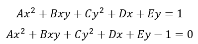
From the above equation we can write in term of general constants:
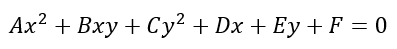
From the equation above, there are five independent variables that describe the ellipse and one constant to define the scale of the ellipse. The value of F is -1
The five independent variables are two variables to define the centre, two variables to define the major and minor axes and one variable to define the tilt angle.
The requirement for the data points to fit the ellipse are:
- The number of points should be oversampled that are more than 5 points. With oversample, the averaging effect obtained from the least square algorithm (will be explained later on) will be obtained to reduce noise on and the bias effect of the point coordinates.
- The points should be distributed around the ellipse to have a better constraint on the ellipse fitting process.
From the equation above, we can form a matrix J, that is a matrix with n-row and 5-column. The i-th row of the matrix J, for each xy-pair of data point, is defined as:
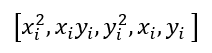
For example, if a data point is (1,2), hence the row will be [1,2,4,1,2].
The next step is by writing the coefficient A,B,C,D,E into a column vector so that we can have a matrix equation (also known as the normal equation) defined as:
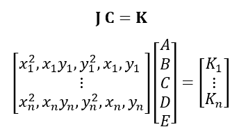
where $K_{1}=K_{2}=...=K_{n}=1$.
To solve the above matrix equation and find the parameter A,B,C,D,E, we apply some matrix algebra operations, such that:
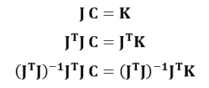
because:
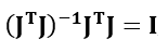
hence:
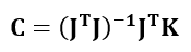
From the final equation above, we can estimate matrix C that contain the fitted parameters: A,B,C,D,E.
Ellipse centre points
After finding the parameters, we must convert these parameters into ellipse parameters: two points centre, major and minor axes and the tilt angle.
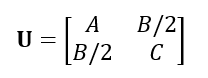
The conversion of parameter A,B,C,D,E to the ellipse parameters are as follows. From the fitted coefficient A,B,C,D,E, we define a matrix U as:
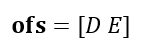
And an offset vector ofs as:
Hence, the ellipse centre points are calculated as:
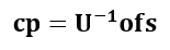
Cp is a vector with two elements, the x- and y- coordinate of the ellipse centre.
Ellipse major and minor axes and tilt angle
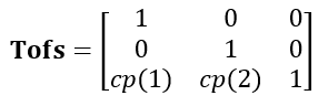
To find the ellipse major and minor axes as well as the ellipse tilt angle, the procedure is as follow. We define a matrix Tofs as:
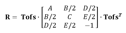
Hence, we calculate matrix R as:
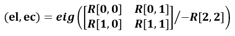
Hence, we calculate matrix el and ec from Eigen value:
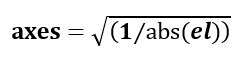
Finally, the major and minor axes (in a form of a matrix) are calculated as:
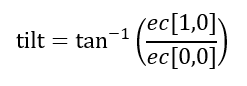
And the tilt angle is calculated as:
C/C++ implementation of the ellipse fitting algorithm with Eigen
The C/C++ implementation, using the Eigen library, of the least-square ellipse fitting as well as deriving the ellipse parameters is presented as follows.
Fitting the general terms (A,B,C,D,E):
float c_x=0,c_y=0,major_axis=0,minor_axis=0,rot_axis=0;

    //STEP 1: Least-square fitting the ellipse polynomial
    MatrixXf poly_coef;
    //poly_coef.resize(5,1);

    MatrixXf K;
    K.resize(pts.size(),1);
    for(int i=0;i<pts.size();i++){
        K(i,0)=1;
    }

    MatrixXf J;
    J.resize(pts.size(),5);
    for(int i=0;i<pts.size();i++){
        float x=0,y=0;
        Point2f pt=pts[i];
        x=pt.x;
        y=pt.y;

        J(i,0)=x*x;
        J(i,1)=x*y;
        J(i,2)=y*y;
        J(i,3)=x;
        J(i,4)=y;
    }

    MatrixXf Jt;
    Jt=J.transpose();

    MatrixXf JtJ;
    JtJ=Jt*J;

    MatrixXf JtJinv;
    JtJinv=JtJ.inverse();

    MatrixXf JtK;
    JtK=Jt*K;

    //least-square fitting process
    poly_coef=JtJinv*JtK;

    float A=0,B=0,C=0,D=0,E=0,F=0;
    F=-1;

    //COEFFICIENT NORMALISATION
    float mag=0.0, tempVal=0.0;
    tempVal=poly_coef(0)*poly_coef(0)+poly_coef(1)*poly_coef(1)+poly_coef(2)*poly_coef(2)+poly_coef(3)*poly_coef(3)+poly_coef(4)*poly_coef(4)+F*F;
    mag=-1*(float)pow(tempVal,0.5);

    poly_coef(0)=poly_coef(0)/mag;
    poly_coef(1)=poly_coef(1)/mag;
    poly_coef(2)=poly_coef(2)/mag;
    poly_coef(3)=poly_coef(3)/mag;
    poly_coef(4)=poly_coef(4)/mag;
    F=F/mag;

    A=poly_coef(0);
    B=poly_coef(1);
    C=poly_coef(2);
    D=poly_coef(3);
    E=poly_coef(4);
Converting the fitted general terms into ellipse parameters (centre point, major and minor axes and tilt angle):
//STEP 2: Derive (convert) the ellipse parameter from the polynomial
    //the algebric form of the polynomial
    MatrixXf Amat;
    Amat.resize(3,3);
    Amat(0,0)=poly_coef(0);Amat(0,1)=poly_coef(1)/2;Amat(0,2)=poly_coef(3)/2;
    Amat(1,0)=poly_coef(1)/2;Amat(1,1)=poly_coef(2);Amat(1,2)=poly_coef(4)/2;
    Amat(2,0)=poly_coef(3)/2;Amat(2,1)=poly_coef(4)/2;Amat(2,2)=F;

    MatrixXf Amat2;
    Amat2.resize(2,2);
    Amat2(0,0)=Amat(0,0);Amat2(0,1)=Amat(0,1);
    Amat2(1,0)=Amat(1,0);Amat2(1,1)=Amat(1,1);

    MatrixXf Amat_inv;
    Amat_inv=Amat2.inverse();

    MatrixXf ofs,cc;
    ofs.resize(2,1);

    ofs(0,0)=poly_coef(3)/2;
    ofs(1,0)=poly_coef(4)/2;

    cc=-1*Amat_inv*ofs;

    c_x=cc(0);
    c_y=cc(1);


   //centre the ellipse at the origin
   MatrixXf Tofs;
   Tofs.resize(3,3);
   Tofs(0,0)=1;Tofs(0,1)=0;Tofs(0,2)=0;
   Tofs(1,0)=0;Tofs(1,1)=1;Tofs(1,2)=0;
   Tofs(2,0)=c_x;Tofs(2,1)=c_y;Tofs(2,2)=1;

   MatrixXf tempM;
   tempM=Amat*Tofs.transpose();

   MatrixXf R;
   R=Tofs*tempM;


   MatrixXf R2;
   R2.resize(2,2);
   R2(0,0)=R(0,0);R2(0,1)=R(0,1);
   R2(1,0)=R(1,0);R2(1,1)=R(1,1);

   float s1=-R(2,2);

   MatrixXf RS;
   RS.resize(2,2);
   //RS=R2/s1;
   RS(0,0)=R2(0,0)/s1;RS(0,1)=R2(0,1)/s1;
   RS(1,0)=R2(1,0)/s1;RS(1,1)=R2(1,1)/s1;


   MatrixXf U;
   VectorXf S;
   MatrixXf V;

   JacobiSVD<MatrixXf> svd(RS, ComputeThinU | ComputeThinV);

   U=svd.matrixU(); //use U or V
   S=svd.singularValues(); //the return values are as a vector (not matrix)!
   V=svd.matrixV();

   float recip1=0, recip2=0;
   recip1=1/fabs(S(0));
   recip2=1/fabs(S(1));


   //STEP 3: Calculating the ellipse major and minor axes and tilt angle
   major_axis=(float)pow(recip1,0.5);
   minor_axis=(float)pow(recip2,0.5);

   float rad=0;
   const float phi=3.14;
   rad=atan(V(1,0)/V(0,0));
   rot_axis=rad*180/phi;
The deployment and distribution of the Qt application for ellipse fitting
This section will explain what files, along with the executable file of the application after compilation, needed to be distributed together with the application file.
There are two types of distributions: distribution of the project source file (if we want to move the development to another computer) and distribution of the executable file (to be run on another computer).
For the project source code distribution:
When we want to move the development environment platform from one computer (PC) to another PC, we need to copy all the project folder containing all the source and Qt project related files.
However, we need to delete a file “*.pro.user” file since this file link all the paths related to compilation and Qt library to our old computer when we do the previous development.
After deleting the “*.pro.user” file, when we open the project main file “*.pro” on a new computer, there will be a prompt window to confirm us the Qt IDE will set the new compiler and all the path related for Qt library automatically.
Finally, we need to set the path for the Eigen and OpenCV libraries in the “.pro” files.
For the executable file distribution:
After the compilation process (in RELEASE mode), we will get the executable file of the ellipse fitting application.
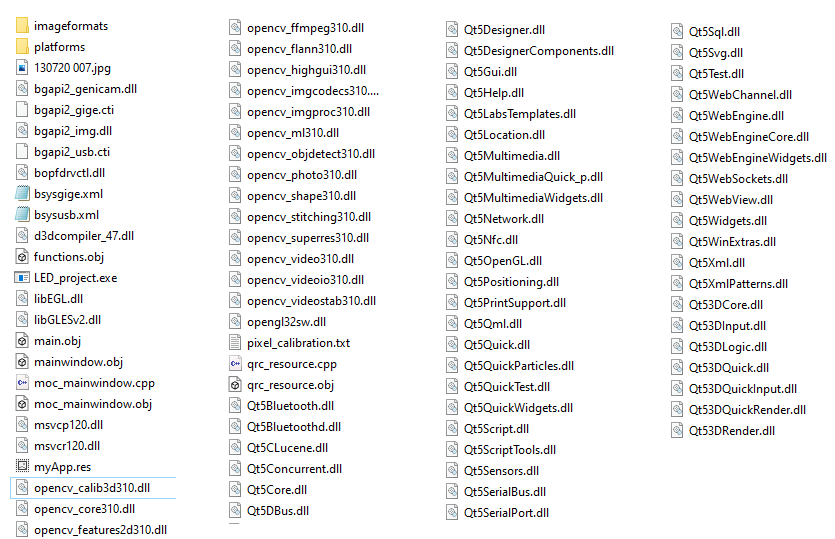
Since the application uses OpenCV and Qt library, the executable files still require dynamic library (“.dll” files) of the OpenCV and Qt library. Hence, all required dynamic link library (DLL) files related to the OpenCV and Qt libraries should be copied into the same folder of the executable file of the application.
For the Qt library, the required DLL files can be found in:
“{Qt_library_installation_path}\{compiler_name}\bin\”
For example:
“{c:\Qt\Qt5.6.3\5.6.3\msvc2015\bin\”
For OpenCV library, the required DLL files can be found in:
“{OpenCV_library_installation_path}\bin\”
Figure 6 shows an example of the DLL files of the Qt and OpenCV in one folder.
Conclusion
In this post, the process flow of developing an ellipse fitting application on Windows operating system is presented. The application is written in C/C++ programming language and uses Qt framework for GUI development, OpenCV for computer vision and Eigen library for matrix and linear algebra operations.
The mathematical equations explaining the least-square ellipse fitting process is presented. The C/C++ implementation of the ellipse fitting uses the Eigen library and is presented in detail.
The image processing procedure, such as image colour conversion, white blobs finding in images, plotting a fitted ellipse and their axes on images and others are explained with their C++ implementation with the OpenCV library.
Finally, the procedure to distribute both the project files and the executable files form one computer to another is also presented in detail.
All the source files, EXE file, include and LIB files as well as documentation of the ellipse fitting in this post can be obtained from this link