Mathematical geometrical fitting: Linear geometry least-squared fitting (with tutorial)
The least-squared fitting of linear geometry is solved by transforming a non-linear objective function of residuals into a linear objective function of the residuals.
The least-squared fitting of linear geometry is solved by transforming a non-linear objective function of residuals into a linear objective function of the residuals.
Readers are suggested to read this “mathematical geometrical fitting: Concept and fitting methods” article beforehand for background.
Linear geometry includes line and plane.
The benefits of transforming a non-linear into a linear objective function is that closed-form mathematical equation can be obtained so that the optimisation can be solved analytically and always gives one global minimum solution.
The transformation process from the non-linear to linear objective functions is performed by using Lagrange method by adding limit function (constraint).
The Lagrange method reduces the linear geometry fitting problems into Eigen value problems. These Eigen value problems have well-known robust solutions so that optimum fitting solutions can be obtained.
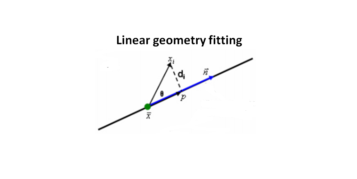
In general, the objective function of linear and non-linear geometry fittings is to minimise the orthogonal distance between measured points and nominal geometry to fit. The definition of the orthogonal distance is different for each type of geometry.
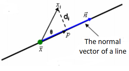
Figure 1 below shows the definition of the residuals of line geometry. It is important that the residuals should be the orthogonal distance so that the distance is independent with respect to the orientation of the line (or other respective geometries).
This orthogonal distance concept applies to all residuals for all different types of geometry to fit.
READ MORE: Mathematical geometrical fitting: Concept and fitting methods
- Numerical Python: Scientific Computing and Data Science Applications - A book Leverage the numerical and mathematical modules in Python and its standard library
Least-squared fitting of plane
The residuals or orthogonal distance between a point to plane is:
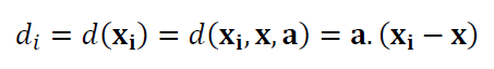
Where $d_{i}$ is the $i$-th residual or the orthogonal distance of $i$-th point to the plane geometry under fitting process. $\bf x$ = $(x,y,z)$ is a point on the plane that is the centroid of all measured points on the plane. $\bf a$=$(a,b,c)$ is the normal vector of the plane, where |$\bf a $|$=1$.
Note that the parameters of the plane that will be estimated from the fitting process is $\bf a$.
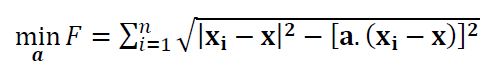
Hence, the objective function for plane fitting is:
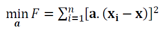
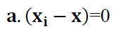
The equation above in this form is a non-linear objective function with the main goal is to minimise the objective function so that:
By applying the Lagrange method [1], the non-linear objective function can be linearised by minimising the Lagrange function with a constraint function.
That is, by applying $F=\lambda G$ with a constraint function of |$\bf a $|$=1$.
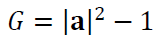
$G$ is a function defined as:
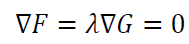
The fitting solution for parameter $\bf a $ that is the minimum value of $F=\lambda G$ can be obtained by applying gradient operator:
So that:
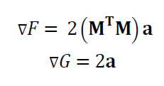
This operation leads to the Eigen value problem (also called the normal equation) as:
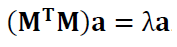
The Eigen vector, representing the parameters to fit $\bf a $, from the equation above can be derived from $\bf M^{T}M$ by applying singular value decomposition (SVD) operation on $\bf M$.
Where $\bf M$ is a $(n \times 3)$ matrix containing the spatial coordinate $(x,y,z)$ of a measured point of which the fitting process will be applied to.
The calculated Eigen vector or $\bf a $ that is the minimum solution of the objective function of the fitting process refers to the smallest Eigen value (resulted from the SVD process).
One important thing to note that there is an ill-condition, that is the plane fitting process is applied to points that is in the same line (colinear).
Hence, plane fitting should be applied to points that are spread across the surface and are not collinear (on the same single line).
The MATLAB code implementation for plane fitting is as follows:
clc;
close all;
clear all;
%POINT GENERATION
%Random error is uniform - function: rand()
% synthetic data generation
nGrid=30;
x=linspace(1,nGrid,nGrid);
y=linspace(1,nGrid,nGrid);
index=1;
for i=1:nGrid
for j=1:nGrid
e=-3+6*randn;
x(i)=i;
y(j)=j;
z(i,j)=x(i)+y(j)+5+e;
%z(i,j)=5+e;
Mraw(index,1)=x(i);
Mraw(index,2)=y(j);
Mraw(index,3)=z(i,j);
index=index+1;
end
end
%LINEAR LEAST-SQUARE PLANE FITTING - NIST ALGORITHM
%NOTE: Translation of the data point to its centroid is compulsary
%Mraw=[x' y' z']; %generate M matrix nx2
MrawHom=Mraw;
MrawHom(:,4)=1;
[n m]=size(Mraw);
avgX=sum(Mraw(:,1))/n;
avgY=sum(Mraw(:,2))/n;
avgZ=sum(Mraw(:,3))/n;
T=[1 0 0 avgX; 0 1 0 avgY; 0 0 1 avgZ; 0 0 0 1];
MtranslatedHom=inv(T)*MrawHom'; %here we have to inverst T from T12 into T21=inv(T12)
MtranslatedHom=MtranslatedHom';
Mtranslated=[MtranslatedHom(:,1) MtranslatedHom(:,2) MtranslatedHom(:,3)];
[U,S,V]=svd(Mtranslated);
%[U,S,V]=svd(Mraw) %WHAT IF the a vector is determined from untranslated data point--> the result is not the same.
singularValue=S(1,1);
a=V(:,1);
for i=2:3
if(singularValue>=S(i,i))
singularValue=S(i,i);
a=V(:,i);
end
end
disp(a);
%Show the fitted/estimated point from the fitting
index=0;
for i=1:nGrid
for j=1:nGrid
x(i)=i;
y(j)=j;
zEstimated(i,j)=((-a(1,1)*(x(i)-avgX)-a(2,1)*(y(j)-avgY))/a(3,1))+avgZ;
end
end
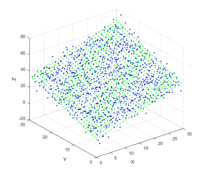
%PLOTTING
[X Y]=meshgrid(x,y);
plot3(X,Y,z,'b.');
xlabel('X');
ylabel('Y');
zlabel('Z');
hold on;
[X2 Y2]=meshgrid(x,y);
plot3(X2,Y2,zEstimated,'g.');
hold on;
grid on;
READ MORE: The fundamental concept of metrology
- Numerical Python: Scientific Computing and Data Science Applications - A book Leverage the numerical and mathematical modules in Python and its standard library
Least-squared fitting of line
The residuals or orthogonal distance between a point to line is:

Where $d_{i}$ is the $i$-th residual or the orthogonal distance (see figure 1 above) of $i$-th point to the line geometry under fitting process. $\bf x$ = $(x,y,z)$ is a point on the line that is the centroid of all measured points on the line. $\bf a$=$(a,b,c)$ is the normal vector of the line, where |$\bf a $|$=1$.
Similar to plane fitting, the $\bf a$ is the parameter of the line that will be estimated from the fitting process.
Hence, the objective function for line fitting is:
By applying the Lagrange method, similar to the plane fitting, the normal equation in term of Eigen value problem is:
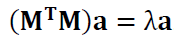
Where $\bf M$ is is a $(n \times 3)$ matrix containing the spatial coordinate $(x,y,z)$ of a measured point of which the fitting process will be applied to and $\bf a$ is the parameters to fit.
However, the solution for $\bf a$ that is the Eigen vector of:

Is the Eigen vector with respect to the biggest Eigen value from SVD operation [1].
In the next post, we will discuss non-linear geometry fitting problems where the objective function to minimised cannot be linearised. Hence, the results of non-linear geometry fitting may not always give optimum results. In addition, the fitting process is in the form of an iteration process (no closed-form mathematical formula that can be solved analytically).
READ MORE: General procedures to operate a tactile coordinate measuring machine (tactile-CMM)
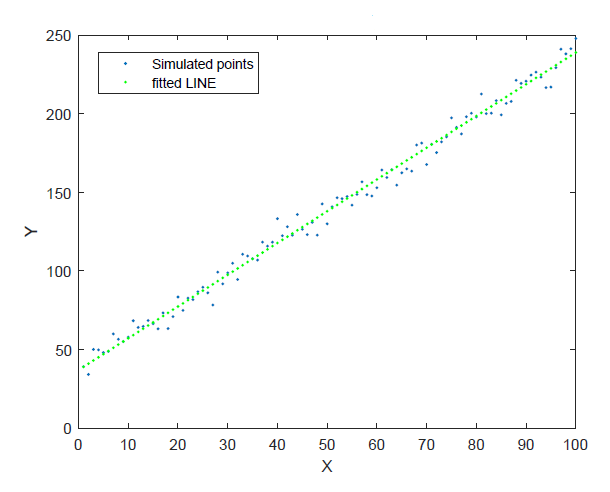
The MATLAB code implementation for 2D line fitting is as follows:
%POINT GENERATION
for i=1:100
    e=-3+6*randn;
    x(i)=i;
    y(i)=2*x(i)+40+e;
end

%LINEAR LEAST-SQUARE 2D LINE FITTING - NIST ALGORITHM
%Translation of the data point to its centroid
Mraw=[x' y']; %generate M matrix nx2
MrawHom=Mraw;
MrawHom(:,3)=1;
[n m]=size(Mraw);
avgX=sum(Mraw(:,1))/n;
avgY=sum(Mraw(:,2))/n;
T=[1 0 avgX; 0 1 avgY; 0 0 1];
MtranslatedHom=inv(T)*MrawHom'; %here we have to inverst T from T12 into T21=inv(T12)
MtranslatedHom=MtranslatedHom';
Mtranslated=[MtranslatedHom(:,1) MtranslatedHom(:,2)];
[U,S,V]=svd(Mtranslated)
%[U,S,V]=svd(Mraw) %WHAT IF the a vector is determined from untranslated data point--> the result is not the same.
if(S(1,1)>S(2,2))
    a=V(:,1)
else
    a=V(:,2)
end
%Show the fitted/estimated point from the fitting
index=0;
for i=1:100
%for i=-50:50
    index=index+1;
    xEstimated(index)=i;
    yEstimated(index)=((xEstimated(index)-avgX)*a(2,1)/a(1,1))+avgY;
end


%PLOTTING
figure(1);
plot(y,'.');
hold on;
%plot(Mtranslated(:,1),Mtranslated(:,2),'r.');
hold on;
plot(xEstimated,yEstimated,'g.');
legend('Simulated points','fitted LINE')
title('NIST Line Fitting Algorithm');
xlabel('X');
ylabel('Y');
zlabel('Z');
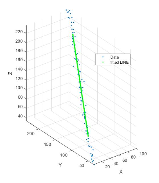
The MATLAB code implementation for 3D line fitting is as follows:
close all;
clear all;
clc;

%POINT GENERATION
for i=1:100
    e=-3+6*randn;
    x(i)=i;
    y(i)=2*x(i)+40+e;
    z(i)=2*x(i)+40+e;
end

%LINEAR LEAST-SQUARE 3D LINE FITTING - NIST ALGORITHM
%Translation of the data point to its centroid
Mraw=[x' y' z']; %generate M matrix nx2
MrawHom=Mraw;
MrawHom(:,4)=1;
[n m]=size(Mraw);
avgX=sum(Mraw(:,1))/n
avgY=sum(Mraw(:,2))/n
avgZ=sum(Mraw(:,3))/n
T=[1 0 0 avgX; 0 1 0 avgY; 0 0 1 avgZ;0 0 0 1];
MtranslatedHom=inv(T)*MrawHom'; %here we have to inverst T from T12 into T21=inv(T12)
MtranslatedHom=MtranslatedHom';
Mtranslated=[MtranslatedHom(:,1) MtranslatedHom(:,2) MtranslatedHom(:,3)];
[U,S,V]=svd(Mtranslated);
%[U,S,V]=svd(Mraw) %WHAT IF the a vector is determined from untranslated data point--> the result is not the same.
singularValue=S(1,1);
a=V(:,1);
for i=2:3
    if(singularValue<=S(i,i))
        singularValue=S(i,i);
        a=V(:,i);
    end
end
a
%Show the fitted/estimated point from the fitting
index=0;
for i=-1000:1000
%Note that the centroid is a point on the line or plane
%Note: 3D-Line --> [x,y,z]=[avgX,avgY,avgZ]+t*[a1,a2,a3]
%where a is direction cosine vector
    index=index+1;
    xEstimated(index)=avgX+(i/10)*a(1);
    yEstimated(index)=avgY+(i/10)*a(2);
    zEstimated(index)=avgZ+(i/10)*a(3);
end

%PLOTTING
figure(1);
plot3(x,y,z,'.');
hold on; grid on; axis equal;
%plot(Mtranslated(:,1),Mtranslated(:,2),'r.');
% hold on;
plot3(xEstimated,yEstimated,zEstimated,'g.');
hold on; grid on; axis equal;
legend('Data','fitted LINE')
title('NIST Line Fitting Algorithm');
xlabel('X');
ylabel('Y');
zlabel('Z');
READ MORE: Research: Lessons learnt from “Hands of Time: A Watchmaker's History of Time”

Conclusion
Linear geometry fitting problems have been discussed in this post. Linear geometries include line and plane geometry or feature.
The fundamental idea of linear geometric fitting is that their non-linear objective function of residuals can be transformed into a linear form by applying Lagrange method with constraint.
With the linearisation, a close loop formula and global optimum solution can be obtained and solved analytically without using an iteration process. That is, the analytical method can obtain the global optimum of parameters that minimised the objective function.
These two basic geometries in many cases very instrumental in obtaining important measurement results.
For example, Features to fit for determining reference coordinate from flat surfaces is plane geometry.
In addition, line fitting is very common, in geometrical and dimensional measurement, to be performed to determine the axis of a cylinder or a symmetrical feature.
Reference
[1] Shakarji, C.M., 1998. Least-squares fitting algorithms of the NIST algorithm testing system. Journal of research of the National Institute of Standards and Technology, 103(6), p.633.
You may find some interesting items by shopping here.
- Numerical Python: Scientific Computing and Data Science Applications - A book Leverage the numerical and mathematical modules in Python and its standard library