Metrology

Mathematical geometrical fitting: Concept and fitting methods

One of instrumental aspects in dimensional, geometrical and surface texture measurements is an algorithm to mathematically fit a geometry to spatial points. These spatial points are captured and digitised by a measuring instrument.

Wahyudin Syam

Jun 29, 2023 • 9 min read

The final value of measurements, such as diameter, flatness, length and other parameters, is derived from a nominal geometry after applying a fitting process to point clouds. This aspect in geometrical and surface texture metrology relates to computer science disciplines.

Fitting algorithms give flexibility of a measuring instrument, such as coordinate measuring machine (CMM), to perform various types of measurement from a set of captured points, called a point cloud.

In this post, the essence of fitting algorithms and their applications will be explained. All readers with or without computer science background can follow this post.

The basic principles of fitting algorithms, for example the definition of the distance between a captured point and the estimation of the point that defines the objective function of the fitting algorithm, will be explained.

The three main point distance definition between a captured point and the estimated point will be discussed. They are maximum total distance, least square and minimum-zone.

Numerical Python: Scientific Computing and Data Science Applications - A book Leverage the numerical and mathematical modules in Python and its standard library

The basic concept of mathematical geometrical fitting process

Fitting algorithm is an instrumental part in the software of a measuring machine, such as CMM. Because, only by this geometrical fitting process, the final value of measurements, for example length, diameter, location and flatness, can be calculated.

Geometrical fitting process is defined as a process to associate a nominal geometry, such as circle or line, to a point cloud by means of minimising the spatial distance between point clouds and the estimated points following a specific objective function [1].

Fitting method is determined by its objective function that minimises residuals. These residuals are the orthogonal distance from a captured point to a nominal geometry or between two geometries, such as planes, circle or cyinder, within which all captured points lie in between.

Commonly, measurement software, such as CMM software, uses least-squared fitting or minimum-zone fitting method to associate (fit) captured (measured) point clouds to a basic nominal geometry.

The selection of whether to use least-square or minimum-zone fitting depends on the type of tolerance verification to performed. Least-squared fitting is suitable for dimensional (classical +/-) tolerance verification and minimum-zone fitting is suitable for geometrical tolerance verification.

Basic geometries are line, plane, circle, sphere, cone and torus [2].

From those basic geometries, they are divided into two classes: Linear geometry and non-linear geometry. Linear geometry includes line and plane. Meanwhile, non-linear geometry includes circle, sphere, cone and torus.

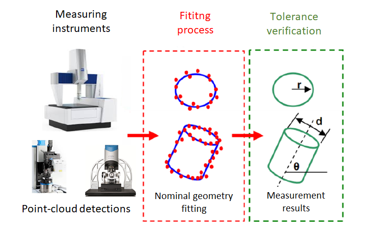
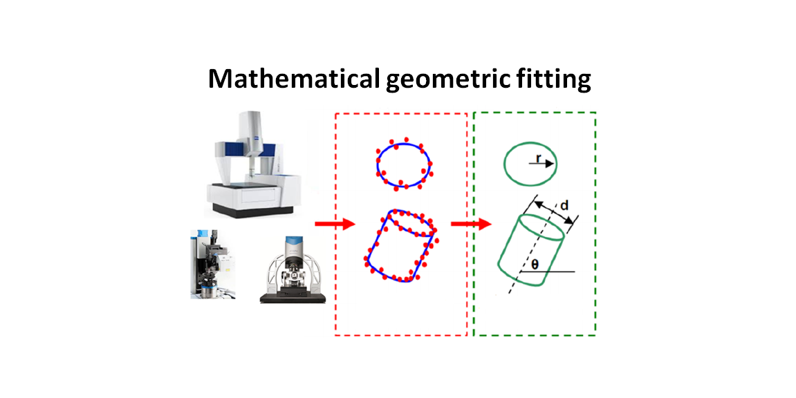
Figure 1: The instrumental role of “mathematical fitting process” in measurement cycle.

Figure 1 above illustrates the instrumental role of geometric fitting process in a measurement cycle. In a measurement cycle, the process begins by collecting or capture points from the surface of a measured part or object and the end of the process obtains a measurement result to be verified with a tolerance specification.

From figure 1, measured points are obtained from a measuring instrument, either contact or non-contact. These points, called point cloud, are then associated to a nominal geometry, such as circle or cylinder by performing a fitting process.

From the fitted nominal geometry, measurement values related to the fitted geometry can be obtained, for example, diameter, depth, height, flatness, circularity, location and others.

Numerical Python: Scientific Computing and Data Science Applications - A book Leverage the numerical and mathematical modules in Python and its standard library

Maximum total distance fitting method

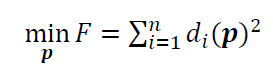
The objective function of maximum total distance method is to minimise the total absolute sum of residuals. As mentioned before, residuals are the distance between a point to its nominal geometry to fit.

This type of fitting is called $L_{1}$ or $l_{1}$ fitting and has median of the residuals that are equal to $0$.

The objective function of maximum total distance fitting is as follow:

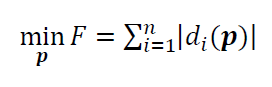
Where $\bf p$ is a vector of parameters of a nominal geometry to fit or to associate point cloud with and $d_{i} (\bf p)$ is the $i-$th residual or the orthogonal distance of measured points to the nominal geometry to fit.

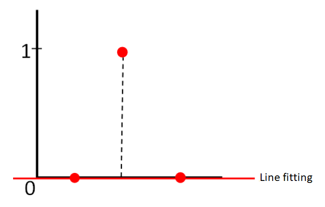
Figure 2 below shows the property of the maximum total distance fitting that is applied to line fitting from three measured points. In figure 2, the minimum of the maximum total distance fitting of the residuals from the three points is $1$, that is when the line passes the two points at the bottom.

Other lines at another position or location will cause the maximum summation of the total distance from the three points to be $> 1$.

For example, if the line is located at the middle of the three points, hence the summation (total) distance of the three points to the line will be $1.5 (>1)$.

Figure 2: An illustration of line fitting based on **maximum total distance** from three measurement points.

The unique characteristic of this maximum total distance fitting is the capability to avoid outliers.

Outliers are defined as points or a set of points that have a very high algebraic distance compared to other points in a point cloud.

This capability to ignore outliers is important to provide final accurate measurement results. for example, when a dust attached to the surface of a measured sphere, the captured points from the dust surface (the outliers) will degrade the quality of the sphere fitting.

This capability is valid if only the number of outliers in the whole point cloud is minority or significantly less than the number of valid points.

By ignoring points due to the dust, the sphere fitting will not be affected and then the measured diameter of the sphere will be accurate.

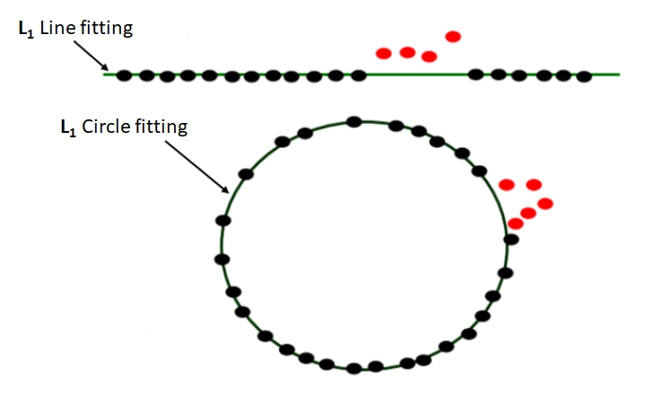
Figure 3 below illustrates the benefit of ignoring outliers’ capability of this fitting method. The outliers are measured points that do not represent the real shape or surface of a part.

In figure 3, examples are shown for robust line and circle fitting where the fitted line and circle are not affected by outliers (red points). Because the outlier points will significantly increase the maximum total distance of the residuals. To minimise the total distance, these outlier points should be ignored to satisfy the objective function of this fitting method.

If the outliers are considered in the fitting process, hence the final geometrical fitting will not represent the real geometry and will lead to invalid measurement results.

Figure 3: An illustration of line and circle fitting based on maximum total distance by ignoring outlier points.

Least-squared fitting method

This least-squared fitting method is the most common fitting method used in measurement. One of the reasons is that there will be an averaging effect from all measures points to a final measurement result.

In this least-square fitting, in an ideal condition, residuals of measured points to a nominal will have a zero average (for unbounded least-square fitting) that is for linear geometry: line and plane fitting. Meanwhile, in an ideal condition for on-linear geometry: circle, sphere, cone and torus, the residuals will not always have zero average.

The other name of least-square fitting is Gaussian fitting or $L_{2}$ or $l_{2}$ fitting.

The objective function of least-square fitting is:

Similarly, where $\bf p$ is a vector of parameters of a nominal geometry to fit or to associate point cloud with and $d_{i} (\bf p)$ is the $i-$th residual or the orthogonal distance of measured points to the nominal geometry to fit.

For linear geometry: line and plane, there will be a single global minimum solution of the objective function. There is a closed-form mathematical model for least-square linear geometry fitting.

However, for non-linear geometry (other than line and plane), there will be several minimum solutions. Usually, iterative optimisation algorithms are required to solve a least-square non-linear geometry fitting task.

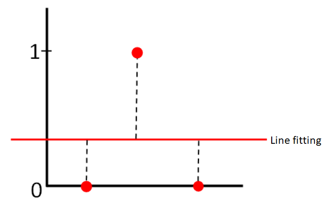
Figure 4: An illustration of line fitting based on **least square** from three measurement points.

Figure 4 above shows the illustration of least-square fitting for line with three measured points. In figure 4, the location of the least-squared fitted line is at 1/3 between the top and bottom points.

Because, only at this location, the total quadratic sum of the residuals is minimum. In principle, the least-squared fitting is the average from the three points.

In other words, least-squared fitting considers all the points without differentiating which one the real points and which one outlier points.

Minimum-zone fitting method

Minimum-zone fitting is also called as min-max fitting or $L_{ \infty}$ or $l_{ \infty}$ fitting.

This minimum-zone fitting is the de facto fitting methodto reconstruct tolerance zone in geometrical tolerance verification (GD&T). The basis of minimum-zone fitting for geometrical tolerance verification is ASME Y14.5.1 [3].

The objective function of minimum-zone fitting is:

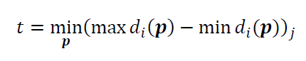
Where $t$ is the distance between two parallel or concentric geometries (could be plane, line, circle, cylinder or sphere) where all measured points located in between the geometries. $\bf p$ is a vector of parameters of a nominal geometry to fit or to associate point cloud with. $d_{i} (\bf p)$ is the $i-$th residual or the orthogonal distance of measured points to the nominal geometry to fit. $j$ is the solution index for each $i-$ point.

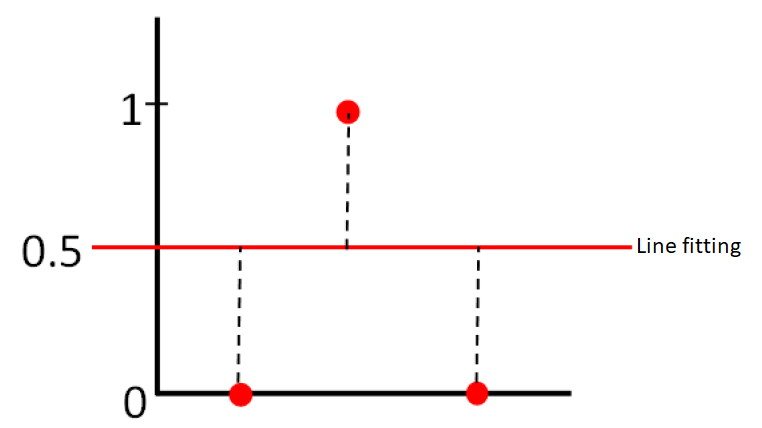
Figure 5: An illustration of line fitting based on **Minimum-zone** from three measurement points.

Figure 5 above shows the illustration of a line fitting based on minimum-zone fitting method from three points. In figure 5, the fitted line is located at ½ distance, that is at the middle, between the above and bottom points.

This line location is because the line located at the middle of two separated paralleled lines. These two separated lines are minimally distanced such that all the three points lie in between the two lines.

In other words, the fitted line lies at the middle of the tolerance zone of the three points defined by the two parallel lines.

An important characteristic of minimum-zone fittingis that this fitting method is only affected by the extreme points or essential points. Other points, that are not at extreme locations, are ignored in the fitting process.

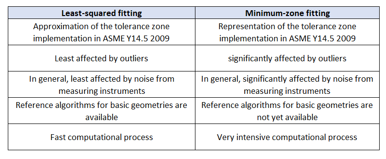
Table 1 below shows the comparison between least-squared and minimum-zone fitting.

Table 1: detailed head-t-head comparison between least-squared and minimum-zone fitting.

Minimum-Circumscribed and Maximum-Inscribed circle/sphere fitting method

Minimum-circumscribed (MC) is a fitting method to fit a circle with minimum diameter in which all measurement points are located within the circle.

Figure 6 below shows the illustration of an MC fitting on measurement points taken by a measuring instrument. In a case where the measurement points have an oval shape, the MC circle will only touch two points that are points at the far-end of the oval shape.

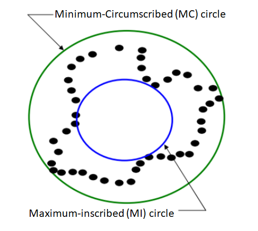
Figure 6: An illustration of circle fitting based on **Minimum-Circumscribed (MC) and Maximum-Inscribed** **(MI)** from measurement points.

Maximum-inscribed (MI) is a fitting method to fit a circle with a maximum diameter where all measurement points are located outside the fit circle or sphere.

Figure 6 above shows the illustration of an MI circle fitting on measured points. One important aspect of MI fitting is that there is a situation where there is more than one MI circle that can fit measured points. That is, the solution may be not unique for a specific set of measured points.

Conclusion

The essence of fitting algorithms and their applications have been presented and discussed in this post. Important concept and fitting methods that are commonly used in the software of measuring instruments have been explained.

There are three main types of fitting methods: maximum total distance, least-squared and minimum-zone fitting. Each of these fitting types has their own specific use in a given measurement task. For example, for geometrical tolerance verification, minimum-zone fitting is used based on ASME Y14.5 standard.

In addition, two specific circle fits are also discussed. These specific circle fits are minimum-circumscribed and maximum-inscribed fitting methods.

Reference

[1] Syam, WP. 2018. “Metrologi Manufaktur: Pengukuran Geometri Dan Analisis Ketidakpastian.” INA-Rxiv. January 4. doi:10.17605/OSF.IO/ZDFXM.

[2] Shakarji, C.M., 1998. Least-squares fitting algorithms of the NIST algorithm testing system. Journal of research of the National Institute of Standards and Technology, 103(6), p.633.

[3] ASME Y14.5-1 1994 Mathematical definition of dimensioning and tolerancing principles American Society of Mechanical Engineering.

You may find some interesting items by shopping here.