Measurement uncertainty estimations: Monte-Carlo simulation method
In this post, a method to estimate measurement uncertainties based on Monte-Carlo simulation is presented with examples.

In this post, a method to estimate measurement uncertainties based on Monte-Carlo simulation is presented with examples.
This Monte-Carlo simulation method is an alternative for measurement uncertainty estimation where GUM method is not applicable. This Monte-Carlo simulation can be used to estimate measurement uncertainty for all types of measurement, for examples, dimensional, geometrical, weight, volume, pressure, viscosity, electric current, velocity and temperature measurements.
Examples used to present the Monte-Carlo method in this post use the exact previous example for measurement uncertainty with GUM in the previous post.
The goal is that direct comparisons of measurement uncertainty estimated by both GUM and Monte-Carlo simulation methods can be performed.
Monte-Carlo simulation: Principle
The Monte-Carlo (MC) simulation method for uncertainty estimation is becoming popular. Because this method is flexible. That is theoretically this method can be used for all types of measurement from simple to very complex measurements, especially when the mathematical model of a measurement is not available.
Particularly, the MC simulation method is very suitable to estimate “Task-specific uncertainty”. “Task specific uncertainty” means that the uncertainty estimation of a measurement result is specific for that particular measurement at that time.
That is, measurement uncertainty is particular for a specific measurement run, environment (temperature, pressure and other factors), measurement parameter, operator, procedure and instrument used for the measurement. A measurement uncertainty of a specific measurement cannot be applied to the same exact measurement performed at a different, for example, place, environment and by a different machine.
One of the weaknesses of this MC simulation method is that this method requires an intensive computation process, especially for complex measurement. However, with the technological advancement and affordability of current available computers, the weakness can be overcome.
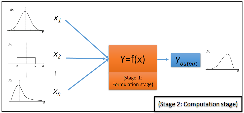
Figure 1 shows the main process flow for MC simulation to estimate measurement uncertainties. From figure 1, the stages for MC simulation are:
1. Formulation stage
On this stage, the formulation of a measurement process is performed. The formulation does not mean to obtain the mathematical model or function of the measurement.
Because, one of the motivation of using the MC simulation is that the mathematical model of the measurement is not required.
The most important thing in this stage is that the measurand (property to measure) of the measurement should be clearly defined.
2. Computation stage
This stage is the essence of the MC simulation method. On this stage, the propagation of uncertainty contributors (following GUM) of a measurement process is performed.
The propagation process is carried out by adding random noise to each variable contributing to the measurement uncertainty. The noise follows a specific probability distribution (with its distribution-defining parameters).
This stage is an iterative calculation process (performed by a computer) and the results from each iteration process is stored in a computer memory. From the stored calculation results, the standard deviation of the results is calculated and is used as an estimate of the measurement uncertainty.
Gaussian and rectangular distributions
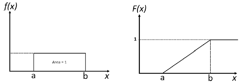
There are two most common distributions used in the MC simulation method. The distributions are Gaussian (normal) and rectangular distribution. Figure 2 and figure 3 show the graphical description (probability density function and cumulative distribution function) for the Gaussian and rectangular distributions, respectively.
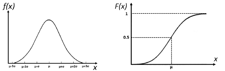
Gaussian distribution
Gaussian distribution is the most common used statistical distribution to generate random variables in any MC-based simulations. These random variables represent various types of uncertainty contributors, for example, temperature variation, pressure variation and the repeatability of and instrument.
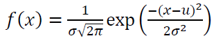
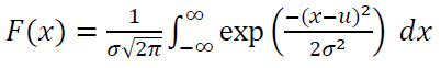
The mathematical model of Gaussian probability density function (PDF) is:
The mathematical model of Gaussian cumulative distribution function (CDF) is:
Rectangular distribution
Rectangular probability distribution is commonly used to generate random variables that represent uncertainties from the resolution of measuring instruments and from the calibration value of calibrated reference artefacts.
The mathematical model of Rectangular probability density function (PDF) is:
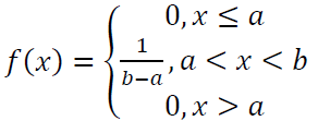
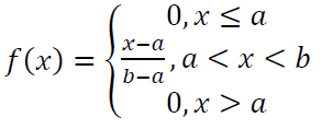
The mathematical model of Rectangular cumulative distribution function (CDF) is:
Monte-Carlo simulation: Procedure and validation
All MC simulation-based measurement uncertainty estimation methods follow the same procedure as shown in figure 1. The general procedure for MC simulation method to estimate the uncertainty of a measurement is as follows:
1. Determine the number of simulations run $n$.
In general, $n$ is a constant variable with a large value, for example, $10^{6}$.
2. Repeat for $n$ times:
2.1 Generate random variables for each uncertainty contributor (input) $X={X_{1}, X_{2},…, X_{n}}$ that are drawn from the probability density function of each contributor $X$, for example, from Gaussian distribution, rectangular distribution or exponential distribution.
2.2 Calculate the measurement output $Y$ according to the mathematical model of the measurement $Y_{i}=f(X_{i})$ if available. When $Y_{i}=f(X_{i})$ is not available, then the measurement output is propagated from data points taken from a real measurement by adding noises to the data points.
3. From all the calculation results (output) from $Y_{i}$ that are repeated for $n$ times:
- If the statistical distribution of the measurement results $Y_{i}$ from the simulation is known (in general, they are assumed as Gaussian distribution), then the standard deviation from $Y_{i}$ is calculated and is used as the estimated uncertainty $u$.
- If the statistical distribution of the measurement results $Y_{i}$ from the simulation is not known and cannot be assumed, then sort all the outputs $Y_{i}$ from the smallest to the largest values (ascending order) to get a sequence $G={Y_{i}, i=1,…,n}$ and take the value $Y_{i}$ from the set $G$ at the position of 2.5% (as the lower limit) and 97.5% (as the upper limit). These two limits are then used as the uncertainty interval (95% confidence interval).
Because MC simulation is a computer-based method, a validation process should be applied to uncertainty estimations based on the MC simulation method.
The validation process for MC simulation-based uncertainty estimation is as follows:
1. Compare the results of uncertainty estimations from an MC simulation with the results based on GUM method (if the mathematical function of a measurement is known). This validation method is not very applicable. Because, very often, we do not have the mathematical model of the measurement (it is one of the main motivations to use the MC simulation method).
2. Compare the results of uncertainty estimations from the MC simulation with the results based on an experimental method that uses a measurement instrument with high accuracy (based on ISO 15530-4).
3. Compare the results of uncertainty estimations from the MC simulation with the results based on a reference software (commonly issued by a national measurement institute/NMI) that uses a reference data with known properties.
Example 1: Measurement uncertainty of length measurement with a Vernier calliper
In this example, we use the same exact Vernier calliper measurement example like the previous example for GUM method.
By using the exact example, we can directly compare the uncertainty estimation method by using the MC simulation method with GUM method.
In this example, the length measurement of a gauge block with Vernier calliper is presented. Figure 4 shows the measurement process.
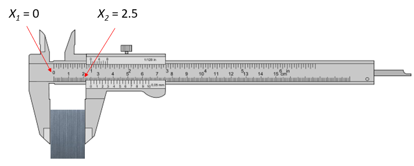
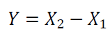
This type of measurement has a very simple measurement model so that this example is very good to explain the uncertainty estimation using GUM and MC simulation methods (the MC simulation method can be compared to the GUM method). The mathematical model of this measurement is:
The implementation of the MC simulation method is in MATLAB codes and is presented below.
From the MATLAB code, the number of iterations for the MC simulation is 10000 runs (iteration). from the mathematical model of the Vernier calliper for length measurement, there are two main uncertainty contributors, that are $X_{1}$ and $X_{2}$.
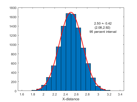
The two contributors are simulated by sampling from Gaussian distribution with mean $0mm$ and standard deviation $0.1 mm$. The calculation results from each iteration $Y_{i}$ is stored so that the total numbers of $Y_{i}$ is 10000 values. From these 10000 values, the standard deviation of $Y_{i}$ is calculated as $0.21mm$.
From this result, the MC simulation results have a very good agreement with the GUM results, that is also $u=0.21mm$.
Figure 5 shows the histogram plot for all calculated $Y_{i}$ on each iteration step of the MC simulation. A Gaussian distribution is fitted and the mean and the standard deviation is calculated and shown.
The MATLAB program for example 1:
clear all;
close all;
clc;

%MC SIMULATION
n=10000;
ux=0.15;
for i=1:n
    x2=2.5+normrnd(0,ux);
    x1=0+normrnd(0,ux);
    Y(i)=x2-x1;
end

%PLOTTING the result
[muhat,sigmahat]=normfit(Y);
Ymin=muhat-2*sigmahat;
Ymax=muhat+2*sigmahat;
text1=sprintf('%.2f +- %.2f\n',muhat,2*sigmahat);
text2=sprintf('(%.2f,%.2f) \n95 percent interval',Ymin,Ymax);
textTotal=sprintf('%s%s',text1,text2);

figure;
histfit(Y,20)
text(Ymax,n/15,textTotal,'HorizontalAlignment','center')
xlabel('X-distance');
Example 2: Measurement uncertainty of profile roughness and waviness
In this example, we use the same exact roughness and waviness measurement examples like the previous example for GUM method(The measurement model and picture are also presented there).
Hence, we also can directly compare the uncertainty estimation method by using the MC simulation method with GUM method.
The waviness and roughness measurement undergo filtering processes. These filtering processes describe the measurement process for waviness and roughness. Figure 6 shows the pictorial description of the waviness and roughness calculations.
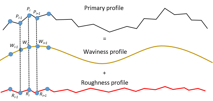
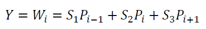
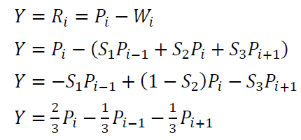
The mathematical model for the filtering process to get the waviness and roughness data are as follow (assuming a rectangular filter with three data point window):
For waviness $W_{i}$:
For roughness $R_{i}$:
The implementation of the MC simulation method for example 2 is in MATLAB codes and is presented below.
Similar with the previous example, the number of iterations of the MC simulation is set to be 10000 runs. From each iteration step, the value of $W_{i}$ and $R_{i}$ are stored so that the number of $W_{i}$ and $R_{i}$ values of are also 10000.
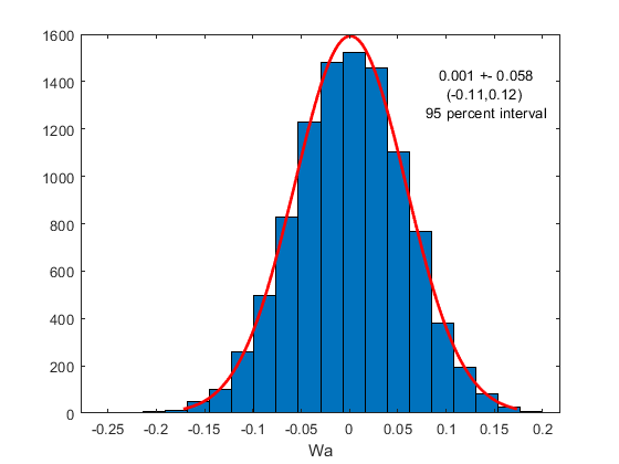
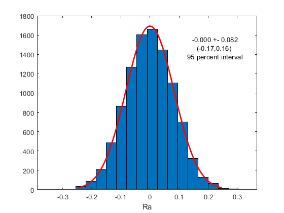
The uncertainty contributors of the roughness and waviness are the uncertainty of the z-position of each point $u_{z}$. The value of $u_{z}$ is simulated by sampling from Gaussian distribution with mean $0\mu m$ and standard deviation $0.1\mu m$.
From the MC simulation, the estimated uncertainty for $W_{i}$ and $R_{i}$ are $0.058\mu m$ and $0.082\mu m$, respectively. By comparing with the results estimated by the GUM method, the uncertainty estimation results from the MC simulation method have a very good agreement with the GUM method.
Figure 7 and figure 8 show the histogram of the values of $W_{i}$ and $R_{i}$ for waviness and roughness, respectively on each iteration step. From the histograms, a Gaussian distribution is fit and its standard deviation is derived.
The MATLAB program for example 2:
clear all;
close all;
clc;

%MC SIMULATION
n=10000;
s=[1 1 1]./3;
uz=0.1;

for i=1:n
    z=zeros(1,19);
    nominal_height = 0;%5;
    z=z+nominal_height;
    z=z+normrnd(0, ones(1,19)*uz);
    %Just estimate the uncertainty of Wa and Ra at one point
    weigth_avg=sum(z(1:size(s,2)).*s);
    W(i)=weigth_avg;
    R(i)=z(2)-W(i);
end

%PLOTTING the result
[muhat,sigmahat]=normfit(W);
Ymin=muhat-2*sigmahat;
Ymax=muhat+2*sigmahat;
text1=sprintf('%.3f +- %.3f\n',muhat,1*sigmahat);
text2=sprintf('(%.2f,%.2f) \n95 percent interval',Ymin,Ymax);
textTotal=sprintf('%s%s',text1,text2);

figure;
histfit(W,20)
text(Ymax,n/15,textTotal,'HorizontalAlignment','center')
xlabel('Wa');

[muhat,sigmahat]=normfit(R);
Ymin=muhat-2*sigmahat;
Ymax=muhat+2*sigmahat;
text1=sprintf('%.3f +- %.3f\n',muhat,1*sigmahat);
text2=sprintf('(%.2f,%.2f) \n95 percent interval',Ymin,Ymax);
textTotal=sprintf('%s%s',text1,text2);

figure;
histfit(R,20)
text(Ymax,n/15,textTotal,'HorizontalAlignment','center')
xlabel('Ra');
From the two examples above, the MC simulation method used to estimate measurement uncertainties is very useful. Because, the MC method can be used for various type of measurements.
Especially, MC method will show its power when the mathematical model of a measurement is not known. Very often, many measurements are complex and their mathematical model is not known or, if known, its mathematical derivation is intractable.
For example, CMM measurements are very common in industries. However, a simple CMM measurement, very often, has an unknown mathematical model because to obtain a value from a CMM measurement, a complex process chain of calculations involved. Hence, the mathematical model cannot be obtained or derived. The MC simulation method can solve this problem.
Conclusion
In this post, the estimation of measurement uncertainty by using Monte-Carlo simulation method is presented. This Monte-Carlo simulation method is an alternative method in cases where the GUM method to calculate measurement uncertainty is not applicable.
The Monte-Carlo simulation can be applied for all types of measurement results, for example, length, volume, velocity, pressure, temperature, weight and humidity measurements.
Real examples, using the previous examples, of uncertainty calculation by using the Monte-Carlo method are shown and explained. The uncertainty estimations from the Monte-Carlo simulation method can be directly compared with the results calculated by GUM method on the exact same examples.
Measurement uncertainty has very important roles in industry and is one of the fundamental concepts in metrology to establish measurement traceability.
We sell all the source files, EXE file, include and LIB files as well as documentation of ellipse fitting by using C/C++, Qt framework, Eigen and OpenCV libraries in this link.
We sell tutorials (containing PDF files, MATLAB scripts and CAD files) about 3D tolerance stack-up analysis based on statistical method (Monte-Carlo/MC Simulation).