Measurement uncertainty estimations: GUM method

Any types of measurement results should be presented with their associated uncertainty. In this post, a method to estimate measurement uncertainties based on Guide to the expression of uncertainty in measurement (GUM) is presented with examples.

GUM is the fundamental reference for uncertainty estimation that is applicable for all types of measurement, for examples, dimensional, geometrical, weight, volume, pressure, viscosity, electric current and temperature measurements.

The principle of GUM is that the uncertainty of a measurement should be calculated by propagating the uncertainty of contributing factors relevant to the measurement. The uncertainty propagation is derived from the model of the measurement.

Contributing factors to measurement uncertainties can be classified into five categories: instrument, operator, work piece, measurement procedure and environment (such as ambient temperature and pressure).

Definition

Uncertainty is a non-negative parameter that represents the dispersion of a quantity associated or attributed to a measurand (VIM). Measurand is a property to be measured, for example, length, mass, volume and temperature.

An uncertainty value represents the amount of the lack of understanding toward a measurement process. In other words, uncertainty is the quantification of our doubt on a measurement.

The smaller the uncertainty value of a measurement, the larger our understanding or knowledge about the measurement.

It is worth to note that "uncertainty" is only associated to a measurement result and not to an instrument. Meanwhile, "error" is associated to an instrument.

Eight general steps to estimate measurement uncertainty

There are various methods to estimate measurement uncertainty. In this post, GUM method is explained.

However, there are eight general steps that should be followed to determine measurement uncertainty regardless of what method is used. The general steps are:

1. Think ahead of time about measurement procedures to follow, what measuring instruments to use and safety aspects during measurement processes.
2. Perform the measurement according to a plan
3. Estimate contributing factors that are relevant to the measurement
4. Consider correlation effects among the contributing factors (commonly the correlations are neglected)
5. Calculate measurement results, including systematic error correction
6. Determine the measurement uncertainty (commonly within 95% confidence interval)
7. Express the measurement results with the confidence interval, determined from the uncertainty
8. Record the measurement results and the uncertainty for future improvement

GUM fundamental formula

GUM method states that the uncertainty of a measurement result must be propagated from the uncertainty of each contributing factor that affects the measurement. To propagate the uncertainty, GUM formula is defined as:

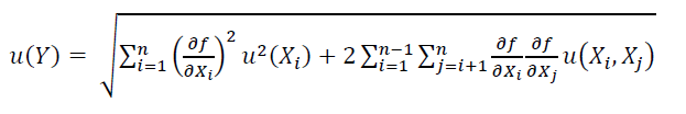
Where $u(Y)$ is the total standard uncertainty value of a measurement $Y$ propagated from its contributing factors. $X_{i}$ is the $i-th$ component of the contributing factors. $u(X_{i},X_{j})$ are the correlation values between “$i$” and “$j$” components.

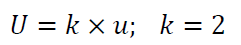
Commonly, uncertainty is presented within 95% confidence interval. This 95% confidence interval uncertainty is called expanded uncertainty $U$. $U$ is formulated as (assuming Gaussian or normal distribution):

From where the formula is derived?

To derive the GUM formula, let us assume that a measurement $y$ is formulated as:

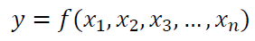
The $y$ above can be linearised by using Taylor expansion method as:

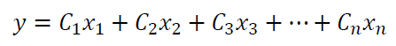
Where $C_{i}$ is the coefficients of Taylor expansion. By applying statistical variation property to the above linearised $y$, we get:

Where $var(cy)=C^{2}\mu ^{2}$, so that:

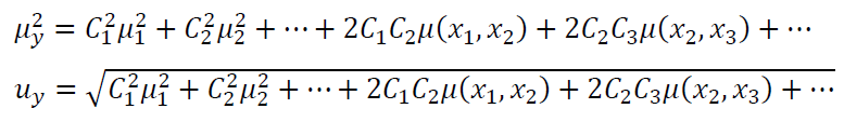
The above equation is the GUM formula as mentioned before. From this equation, GUM method requires a mathematical model that describes a measurement.

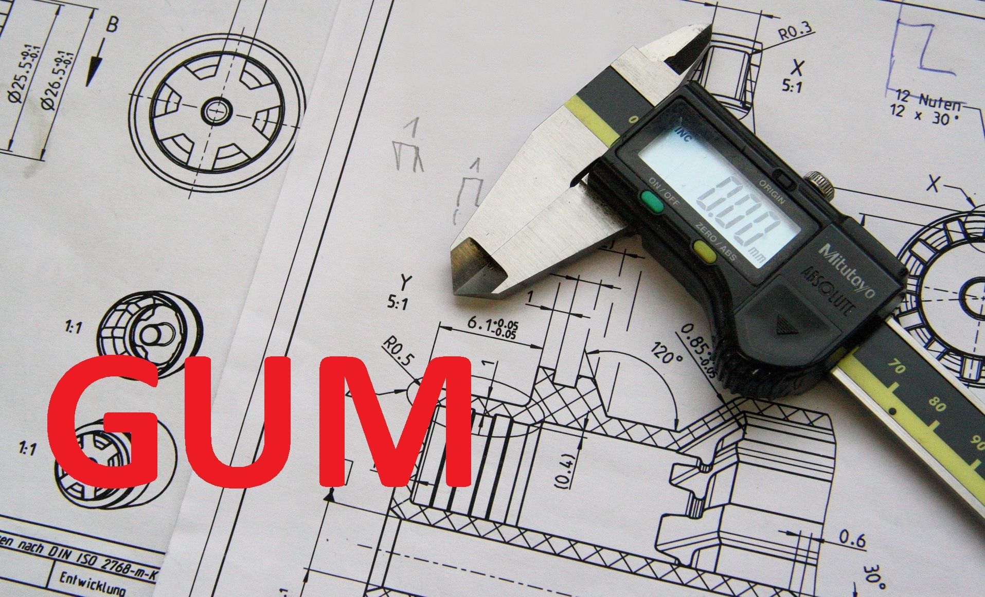
Example 1: A Vernier Calliper measurement

In this example, the simplest measurement process is presented. The example is the length measurement of a gauge block by using a Vernier Calliper.

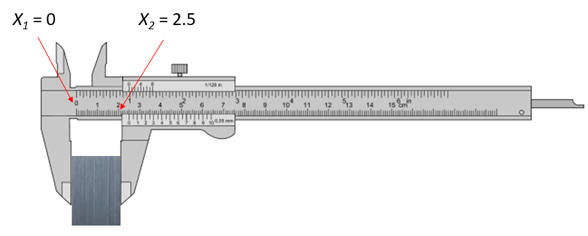
The measurement process is shown in figure 1. From figure 1, the length measurement is defined as the difference between two measuring scales read from the Vernier Calliper. Hence, the measurement model is formulated as:

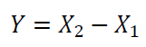
Where $X_{1}$ and $X_{2}$ are the two scales read from the calliper. In this case, temperature effect is neglected and not included in the model.

From the measurement (figure 1), we can observe that $X_{1}=0 mm$ and $ X_{2}=2.5 mm$. Hence, the gauge block’s length $Y=2.5 mm$.

By applying GUM method to estimate the uncertainty, we can derive:

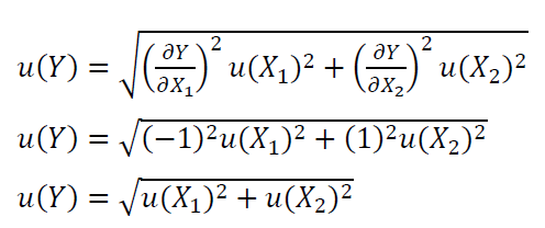
Assuming that the uncertainties from all the contributors are equal $X_{1}$ =X_{2}=0.1 mm$. These values are obtained from the previous calliper calibration process and the correlation effect is neglected.

Hence, the uncertainty of the measurement is:

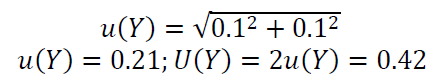
Where $U(Y)$ is the expanded uncertainty with 95% confidence interval ($k=2$).

Finally, the length measurement result is presented as:

• The gauge block length = $Y=(2.5\pm 0.42) mm$
• The 0.42 interval is the expanded uncertainty $U$ with expansion factor $k=2$ that covers 95% confidence interval.
• The length 2.5 mm is the average from five measurement repetitions. The expanded uncertainty is estimated by using GUM method. The measurement was carried out at the shop floor at $(25\pm 0.4)$ degree Celsius by an experience operator.

Readers may read this post regarding how to correctly present a measurement result.

Example 2: Profile roughness and waviness measurements

In this example, the point uncertainty from roughness profile data is presented.

Roughness and waviness are surface texture parameters that are calculated from surface data after filtration processes to remove the form components on the surface data. For example, if we measure the surface of a ball, the raw data points will have a sphere shape. This sphere shape is the form that needs to be filtered to get the roughness and waviness data.

When the form data of the sphere have been separated, the data points will become flat because the form components have been removed. After the form removal, the primary profile of the surface data can be obtained.

From this primary profile, with further filtering processes, the roughness and waviness of the surface can be calculated.

Roughness is calculated by applying a high-pass filter to primary profile data. That is, roughness only considers high frequency data. From this roughness data, roughness parameters, such as $R_{a}, R_{q}$, can be calculated.

Waviness is calculated by applying a low-pass filter to primary profile data. That is, waviness only considers low frequency data.

Figure 2 shows filtering processes applied to primary profile data. From the filtering processes, two different scales of data can be obtained: waviness profile and roughness profile.

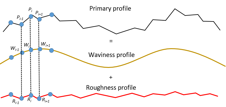
In this example, the uncertainty of a roughness and waviness points are presented. In this example, three points from the primary profile ($P_{i}$), filtered to obtain the waviness point (W_{i}) and roughness point ($R_{i}$) are considered for the calculation examples.

Uncertainty of a waviness point

We assume a rectangular filter is used to separate primary profile data into waviness profile data. The rectangular filter contains three elements ($S_{1}, S_{2}, S_{3}$).

Each filter element $S_{i}$ has a weight of 1/3, so that $S_{1}= S_{2}= S_{3}$=1/3. The waviness point $W_{i}$ is calculated as weighted average from the primary profile data calculated with the rectangular filter.

The mathematical function or model to get a waviness point $W_{i}$ is:

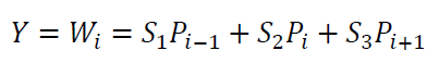
Where $W_{i}$ is the $i-th$ data point of the waviness profile (figure 2) obtained by applying the filter to the primary profile.

Hence, the uncertainty of $W_{i}$ by using GUM method is calculated as:

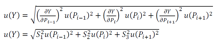
We assume that the uncertainty value for each primary data point $u(P_{i-1}=u(P_{i})=u(P_{i+1})=u(P))=0.1 \mu m$. This uncertainty value can be calculated, for example, from the point repeatability from measurement repetitions.

Hence, the total standard uncertainty $u(Y)$ is:

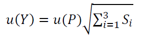
So that:

Note that if we compare the uncertainty between $W_{i}$ and $P_{i}$, we will observe that $u(W_{i})<u(P_{i})$. This reason is that there is an averaging effect from the filtering process when we calculate the $W_{i}$ points.

Uncertainty of a roughness point

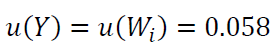
From the same primary profile $P_{i}$ and the rectangular filtering value as the previous waviness example, the uncertainty of $R_{i}$, that is $u(R_{i})$ is calculated.

The mathematical model to get the $R_{i}$ points is (see figure 2):

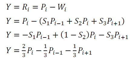
By applying GUM method, the total standard uncertainty $u(Y_{i})=u(R_{i})$ is:

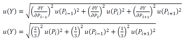
The same as before for the case of the waviness, we assume that the uncertainty value for each primary data point $u(P_{i-1}=u(P_{i})=u(P_{i+1})=u(P))=0.1 \mu m$ and $S_{1}= S_{2}= S_{3}=1/3$. By neglecting correlation effects, we get:

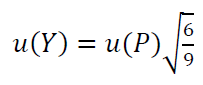
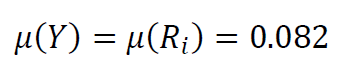
So that, $u(Y_{i})=u(R_{i})$ is:

Example 3: A depth measurement by a sonar system

In this example, a depth measurement by using a sonar system is presented. A sonar system is a system that uses sound propagations to measure distances (mostly depth), detect objects and navigate vessels and submarines.

The measurement model for the depth measurement is:

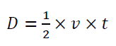
Where $D$ is the measured depth, $v$ is the sound velocity originated from the sonar system and $t$ is the sound travel time from being transmitted from to receive at the transducer of the sonar system.

From the measurement model above, the contributing factors for the depth measurement uncertainty $D$ are $v$ and $t$.

In addition, another uncertainty contributor is the depth accuracy that is dependent to every measured D. Hence, there are a total of three uncertainty contributors.

The uncertainty propagation model is:

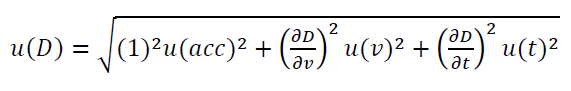
Where:

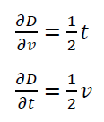
Note that the unit of $\frac{\partial D}{\partial v}$ is $s$ and $ \frac{\partial D}{\partial t}$ is $m/s$. Note that, these partial derivatives (also called coefficient of sensitivity) convert the unit of $u(v)$, having unit of $m/s$, and $u(t)$, having unit of $s,$ to $m$.

$u(acc)$ is the uncertainty that is dependent to every measured $D$ and the instrument characteristics (obtained from the manufacturer data sheet). From the datasheet, $u(acc)=0.00005 m$

After calculation from the data, $u(v)=1.485m/s$ and $u(t)=3.3 \times 10^{-7}s$ are obtained.

After knowing the $u(acc), u(v), u(t)$, we can calculate the total standard uncertainty of $D$ by using GUM uncertainty propagation model for the sonar depth measurement above.

The estimated $u(D)$ is $0.0025m$ and the expanded uncertainty is $U(D)=0.05m$ with $k=2$.

The disadvantages of GUM method

Although GUM method is the main reference to follow in determining measurement uncertainty for all types of measurements, this method has several drawbacks that are not always applicable in practice. Some drawbacks of GUM method are:

• Require the analytical or mathematical model of a measurement. In practice, most of real measurements are complex and their analytical measurement models are not available (if not difficult to derive). If the measurement models are not available, we cannot apply partial derivate, required by GUM method, to propagate the uncertainties of contributing factors of the measurement.
• Require function partial derivations of a measurement model. Although the mathematical model of a measurement is available, very often, the model cannot be partially derived.
• Require a complex modelling and calculation, even for simple measurements. The complex modelling and calculation can be a barrier for industrial application or industrial use.

Conclusion

In this post, GUM method to estimate measurement uncertainties is presented. The GUM is the main reference to calculate measurement uncertainty for all types of measurement results, for example, length, volume, pressure, temperature, weight and humidity measurements.

Three real examples of uncertainty calculation by using GUM method are shown and explained. The examples show in detailed how measurement processes are modelled and how their measurement uncertainties are estimated.

Measurement uncertainty is one of the fundamental concepts in metrology and has important roles in industry.

We sell all the source files, EXE file, include and LIB files as well as documentation of ellipse fitting by using C/C++, Qt framework, Eigen and OpenCV libraries in this link.

We sell tutorials (containing PDF files, MATLAB scripts and CAD files) about 3D tolerance stack-up analysis based on statistical method (Monte-Carlo/MC Simulation).