TUTORIAL: C/C++ implementation of circular buffer for FIR filter and GNU plotting on Linux
In this post, a tutorial for implementing the concept of circular buffer to a finite impulse response (FIR) filtering application of continuous data is presented. Also, the plotting of the filtered data with GNU plot application in Linux will be shown.
In this post, a tutorial for implementing the concept of circular buffer to a finite impulse response (FIR) filtering application of continuous data is presented. Also, the plotting of the filtered data with GNU plot application in Linux will be shown.
The implementation uses C/C++ programming language under Linux operating system. The plotting is performed by sending data to the GNU plot application (as one of default application in Linux) with a piping method.
Piping operation in Linux is an operation (in term of a command) that redirects the standard output, input, and error of a process (program) to another different process (program). The commands for opening and closing a piping process (popen() and pclose() respectively) are included in <stdio.h>header file in Linux.
FIR filter is a filter that has a finite impulse response duration. Meaning, the filter will settle to zero at a finite time. A very common application of FIR filter is for removing high frequency noise, that is as a low-pass filter.
Circular buffer is a type of data structure in the form of a single fixed-size buffer connected end-to-end (cyclic). The use of circular buffer for continuous data streams buffering is to speed up a computation that requires inputs from previous processes or outputs for real-time applications. Other names that refer to circular buffer are ring buffer, circular queue or cyclic buffer.
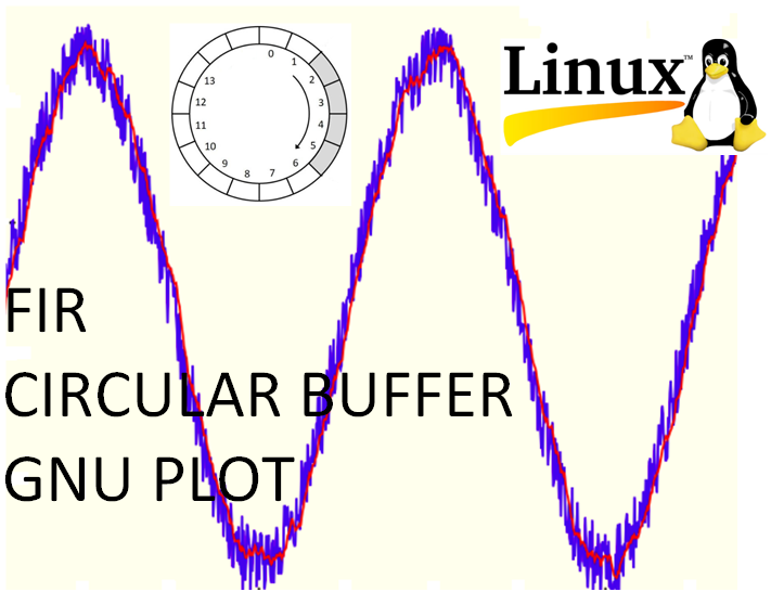
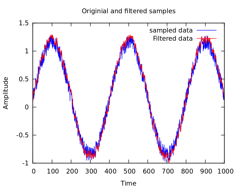
At the end of this tutorial, we will be able to filter noisy data and plot the data for visualising the results. Figure 1 shows the results we will get after following this tutorial. In figure 1, the plot shows the data before and after filtering as well as the legend explaining the curve type based on the colours.

Let us go into the details!
(It is worth to note that we need to beware of integer data type in computing. You may also interested to read other tutorials for applied programming)
File structure and folder directory
Before going to the detailed steps for the tutorial, it will be good if we know what files are involved in this tutorial as well as their folder arrangement.
Note that the arrangement of the files, in term of what folder they are in, is flexible depending on our desire. However, the file and folder arrangements shown here are the common practice for C/C++ developers.
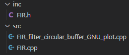
Figure 2 shows the structure of files and folders involved in this tutorial. In figure 2, there are two folders:
- Inc: to include the header file of the FIR filter. This folder contains one file: “FIR.h” as the header file of the FIR filter.
- Src: to include the main source file and the FIR filter implementation. This folder contains “FIR_filter_circular_buffer_GNU_plot.cpp” as the main file and “FIR.cpp” as the FIR filter implementation.
FIR filter header and source code implementation files
The FIR filter is implemented in other files separated from the main .CPP file (FIR_filter_circular_buffer_GNU_plot.cpp). The reason is that we can localise the functions so that the functions can be independently modified to reduce the program complexity.
The FIR filter is composed of a header file “FIR.h” and implementation “FIR.cpp”. These two files are explained as follow:
Header file
In C/C++, the header file “.h” usually contains only the definition of data types and function (usually called function prototypes). In this case study, the header file contains the definition of:
- A struct data type of FIRFilter.
- Two function prototypes (declaration): FIRFilter_init()and FIRFilter_calc().
The code for the “FIR.h” is as follow:
#ifndef FIR_FILTER_H
#define FIR_FILTER_H

#include <stdint.h>

#define FIR_FILTER_LENGTH 5

//Defining the struct to represent the circular buffer
typedef struct{
    float buff[FIR_FILTER_LENGTH]; //for circular buffer array
    uint8_t buffIndex; //Tracking the index of the circular buffer
    float out; //the output value of the circular buffer
} FIRFilter;

//functions prototype
void FIRFilter_init(FIRFilter *fir);
float FIRFilter_calc(FIRFilter *fir, float inputVal);

#endif
The directives:
#ifndef FIR_FILTER_H
#define FIR_FILTER_H
#endif
are used to avoid double declaration of data types, functions or other included libraries. This practice is recommended for C/C++ header files.
Source code implementation files
The mathematical formula for FIR filter is a weighted sum of recent and previous inputs (depending on the filter length). The FIR filter is formulated as:
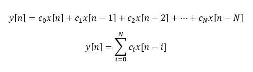
Where:
$x[n]$ is the $n$-th input signal
$y[n]$ is the $n$-th output signal that is the filter output
$N$ is the filter order. An $N$-th order filter will require $N+1$ input value to calculate the output $y$.
$c_{i}$ is the filter coefficient that is the impulse response of the filter at an $i$-th instant.
The filter coefficient $c_{i}$ is determined from a filter design process. These coefficients determine the behaviour of the filter (for example as a low-pass filter).
The final implementation of the FIR filter in C/C++ code for the “FIR.cpp” is as follow:
#include "FIR.h"

//define the variable in the stack memory, including declaration. The value of this
//FIR_FILTER_IMPULSE_RESPONSE array is based on a design (the value represent the behaviour of the filter)
static float FIR_FILTER_IMPULSE_RESPONSE[FIR_FILTER_LENGTH]={0.4,0.3,0.2,0.1,0.05};

//function to initialise the circular buffer value
void FIRFilter_init(FIRFilter *fir){ //use pointer to FIRFilter variable so that we do not need to copy the memory value (more efficient)
    //clear the buffer of the filter
    for(int i=0;i<FIR_FILTER_LENGTH;i++){
        fir->buff[i]=0.0f;
    }

    //Reset the buffer index
    fir->buffIndex=0;

    //clear filter output
    fir->out=0.0f; //'f' to make is as a float
}

//function to calculate (process) the filter output
float FIRFilter_calc(FIRFilter *fir, float inputVal){

    float out=0.0f;

    /*Implementing CIRCULAR BUFER*/
    //Store the latest sample=inputVal into the circular buffer
    fir->buff[fir->buffIndex]=inputVal;

    //Increase the buffer index. retrun to zero if it reach the end of the index (circular buffer)
    fir->buffIndex++;
    uint8_t sumIndex=fir->buffIndex;
    if(fir->buffIndex==FIR_FILTER_LENGTH){
        fir->buffIndex=0;
    }

    //Compute the filtered sample with convolution
    fir->out=0.0f;
    for(int i=0;i<FIR_FILTER_LENGTH;i++){
        //decrese sum index and warp it if necessary
        if(sumIndex>0){
            sumIndex--;
        }
        else{
            sumIndex=FIR_FILTER_LENGTH-1;
        }
        //The convolution process: Multyply the impulse response with the SHIFTED input sample and add it to the output
        fir->out=fir->out+fir->buff[sumIndex]*FIR_FILTER_IMPULSE_RESPONSE[i];
    }

    //return the filtered data
    return out;

}
Circular buffer concept and implementation
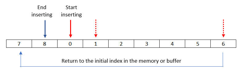
A circular buffer is implemented in memory as a linear array. Figure 3 shows the illustration of a circular buffer.
In figure 3, the starting location to insert a value on the buffer can be from any array indexes. When a new input value arrives, the index location to insert the new value will be on the next array index. If the array index reaches the maximum array size, then the index location will be re-started from the beginning of the array (hence becomes circular).
The code section implementing the circular buffer is as follow:
/*Implementing CIRCULAR BUFER*/
    //Store the latest sample=inputVal into the circular buffer
    fir->buff[fir->buffIndex]=inputVal;

    //Increase the buffer index. retrun to zero if it reach the end of the index (circular buffer)
    fir->buffIndex++;
    uint8_t sumIndex=fir->buffIndex;
    if(fir->buffIndex==FIR_FILTER_LENGTH){
        fir->buffIndex=0;
    }
From the code section above when an input value arrives, the buffIndex is added to 1 (to go to the next array index). If the buffIndex is equal to FIR_FILTER_LENGTH (the FIR filter length), hence the buffIndex is reset to zero again.
The calculation of the FIR filter output using the circular buffer is in the code section below:
//Compute the filtered sample with convolution
    fir->out=0.0f;
    for(int i=0;i<FIR_FILTER_LENGTH;i++){
        //decrese sum index and warp it if necessary
        if(sumIndex>0){
            sumIndex--;
        }
        else{
            sumIndex=FIR_FILTER_LENGTH-1;
        }
        //The convolution process: Multyply the impulse response with the SHIFTED input sample and add it to the output
        fir->out=fir->out+fir->buff[sumIndex]*FIR_FILTER_IMPULSE_RESPONSE[i];
    }
For the above section of code, following the equation above, the filter output is calculated as the summation of the latest (recent) input value multiplied by the first filter weight and with the input value before the latest one multiplied by the second filter weight and …. until the oldest $n-N$-th input value (the oldest) multiplied with the last weight of the filter.
The main function file
The main file contains the step for the noisy data generation, filtering and plotting. This function will include the FIR filter from the other file “FIR.h” that is linked to “FIR.cpp”.
Each step of the process will be explained in the following sub-section.
The code for the main file “FIR_filter_circular_buffer_GNU_plot.cpp” is as follow:
#include <stdio.h>
#include <stdlib.h>
#include <math.h>

#include "FIR.h" //including the FIR filter functions

int main(int argv, char* argc[]){

    //////////////////// Generating noisy data to be filtered //////////////////////////////////////
    int n=1000;
    float input[n];
    float filteredInput[n];

    //Generate the input values
    const float pi=3.14159265358979;
    const float f=2.5; //Hz
    for(int i=0;i<n;i++){
        float min=0.0f;
        float max=0.3f;
        float noise=min+((float)rand()/(float)RAND_MAX)*(max-min);
        input[i]=(float)sin(2*pi*f*i/n)+noise; //one cycle t=i/n=0 to 1
    }


    //////////////////////// FIR filter with circular buffer//////////////////////////////////////

    //Declaring the filter struct variable
    FIRFilter fir;

    //Initialise the filter coefficient (the weight)
    FIRFilter_init(&fir);

    //Calculating the filtered values
    for(int i=0;i<n;i++){
        FIRFilter_calc(&fir, input[i]);
        filteredInput[i]=fir.out;
    }


    /////////////////////// GNU plotting//////////////////////////////////////////////////////////

    //Plotting with GNU Plot
    FILE *gnuplot;
    char gnuPlotCommandString[500]="";
    char title[200]="";
    char xLabel[200]="";
    char yLabel[200]="";

    //Select and Set the gnulot term for setting the terminal or plot size
    const int NUM_TERMS=5; //from 0 to 4

    //#define NUM_TERMS=5; //from 0 to 4
    char gnuplotTerms[NUM_TERMS][50]={"wxt","x11","qt","fail"};

    //select and get the term type, otherwise fail and out
    int termNo=0;
    for(termNo=0;termNo<NUM_TERMS;termNo++){
        sprintf(gnuPlotCommandString,"gnuplot -e \"set term %s\" 2>1",gnuplotTerms[termNo]);
        gnuplot=popen(gnuPlotCommandString,"r");
        char tempc;
        tempc=fgetc(gnuplot);
        if(feof(gnuplot)){
            break;
        }
        if(tempc) //do nothing. supressing the compiler warning for unused compiler
        fclose(gnuplot);
    }
    if(termNo==4){ //The term option is not available
        char strError[100];
        sprintf(strError,"Cannot find a suitable terminal type for GnuPlot, please ensure gnuplot-x11 is installed");
        printf("[ERROR]: %s\n", strError);
        exit(-1);
    }

    //Open the gnuplot for writing/plotting
    sprintf(gnuPlotCommandString, "gnuplot -persistent 2> /dev/null");
    if ( (gnuplot = popen(gnuPlotCommandString, "w")) == NULL){
        char strError[100];
        sprintf(strError,"Failed to open gnuplot executable");
        printf("[ERROR]: %s\n", strError);
        exit(-1);
    }

    //Set the plot title, xlabel and ylabel
    sprintf(title, "Originial and filtered samples");
    sprintf(xLabel, "Time");
    sprintf(yLabel, "Amplitude");

    fprintf(gnuplot, "set terminal %s size 500,400\n", gnuplotTerms[termNo]);
    fprintf(gnuplot, "set title '%s'\n", title);
    fprintf(gnuplot, "set xlabel '%s'\n", xLabel);
    fprintf(gnuplot, "set ylabel '%s'\n", yLabel);

    //Plot the data
    fprintf(gnuplot,"plot '-' w lines lc rgb 'blue' title \"sampled data\", '-' w lines lc rgb 'red' title \"Filtered data\" ");
    for(int i=0;i<n;i++){
        fprintf(gnuplot,"%d %lf\n",i,input[i]);
    }
    fprintf(gnuplot,"e\n");
    for(int i=0;i<n;i++){
        fprintf(gnuplot,"%d %lf\n",i,filteredInput[i]);
    }

    //Close the GNU plot piping
    fflush(gnuplot);
    fclose(gnuplot);

}
Noisy data generation
This data generation is to create a noisy sinusoid signal to be filtered by the FIR filter. In this code section, the $f$ is the frequency of the sinusoid that we want to generate.
The noise sinusoid data generation is:
input[i]=(float)sin(2*pi*f*i/n)+noise;
In the main file “FIR_filter_circular_buffer_GNU_plot.cpp”, the section for data generation is as follows:
//////////////////// Generating noisy data to be filtered //////////////////////////////////////
    int n=1000;
    float input[n];
    float filteredInput[n];

    //Generate the input values
    const float pi=3.14159265358979;
    const float f=2.5; //Hz
    for(int i=0;i<n;i++){
        float min=0.0f;
        float max=0.3f;
        float noise=min+((float)rand()/(float)RAND_MAX)*(max-min);
        input[i]=(float)sin(2*pi*f*i/n)+noise; //one cycle t=i/n=0 to 1
    }
FIR filter implementation
After generating the noisy signals, we then filter the signal (real time) by sending the each signal value to the FIRFilter_calc() so that the value will be used as a new input to calculate a new filter output.
In the main file “FIR_filter_circular_buffer_GNU_plot.cpp”, the section for FIR filtering is as follows:
//////////////////////// FIR filter with circular buffer//////////////////////////////////////

    //Declaring the filter struct variable
    FIRFilter fir;

    //Initialise the filter coefficient (the weight)
    FIRFilter_init(&fir);

    //Calculating the filtered values
    for(int i=0;i<n;i++){
        FIRFilter_calc(&fir, input[i]);
        filteredInput[i]=fir.out;
    }
From the code section above, we need first to define the struct object “fir” form the struct “FIRFilter”. After defining the object struct, we then can use all the FIR filter functionality.
GNU plotting on Linux
Finally, after the noisy signal is filtered. We then can plot the noisy and the filter signals for visualisation. The plotting use GNU plot that is available native in Linux operating system.
In the main file “FIR_filter_circular_buffer_GNU_plot.cpp”, the section for GNU plotting is as follows:
/////////////////////// GNU plotting//////////////////////////////////////////////////////////

    //Plotting with GNU Plot
    FILE *gnuplot;
    char gnuPlotCommandString[500]="";
    char title[200]="";
    char xLabel[200]="";
    char yLabel[200]="";

    //Select and Set the gnulot term for setting the terminal or plot size
    const int NUM_TERMS=5; //from 0 to 4

    //#define NUM_TERMS=5; //from 0 to 4
    char gnuplotTerms[NUM_TERMS][50]={"wxt","x11","qt","fail"};

    //select and get the term type, otherwise fail and out
    int termNo=0;
    for(termNo=0;termNo<NUM_TERMS;termNo++){
        sprintf(gnuPlotCommandString,"gnuplot -e \"set term %s\" 2>1",gnuplotTerms[termNo]);
        gnuplot=popen(gnuPlotCommandString,"r");
        char tempc;
        tempc=fgetc(gnuplot);
        if(feof(gnuplot)){
            break;
        }
        if(tempc) //do nothing. supressing the compiler warning for unused compiler
        fclose(gnuplot);
    }
    if(termNo==4){ //The term option is not available
        char strError[100];
        sprintf(strError,"Cannot find a suitable terminal type for GnuPlot, please ensure gnuplot-x11 is installed");
        printf("[ERROR]: %s\n", strError);
        exit(-1);
    }

    //Open the gnuplot for writing/plotting
    sprintf(gnuPlotCommandString, "gnuplot -persistent 2> /dev/null");
    if ( (gnuplot = popen(gnuPlotCommandString, "w")) == NULL){
        char strError[100];
        sprintf(strError,"Failed to open gnuplot executable");
        printf("[ERROR]: %s\n", strError);
        exit(-1);
    }

    //Set the plot title, xlabel and ylabel
    sprintf(title, "Originial and filtered samples");
    sprintf(xLabel, "Time");
    sprintf(yLabel, "Amplitude");

    fprintf(gnuplot, "set terminal %s size 500,400\n", gnuplotTerms[termNo]);
    fprintf(gnuplot, "set title '%s'\n", title);
    fprintf(gnuplot, "set xlabel '%s'\n", xLabel);
    fprintf(gnuplot, "set ylabel '%s'\n", yLabel);

    //Plot the data
    fprintf(gnuplot,"plot '-' w lines lc rgb 'blue' title \"sampled data\", '-' w lines lc rgb 'red' title \"Filtered data\" ");
    for(int i=0;i<n;i++){
        fprintf(gnuplot,"%d %lf\n",i,input[i]);
    }
    fprintf(gnuplot,"e\n");
    for(int i=0;i<n;i++){
        fprintf(gnuplot,"%d %lf\n",i,filteredInput[i]);
    }

    //Close the GNU plot piping
    fflush(gnuplot);
    fclose(gnuplot);
from the above code section, to plot the data with GNU plot, we need to send all the data that we want to plot to GNU plot program via piping.
This data transfer uses “popen()” function, natively available in Linux “stdio.h” header file.
The “popen()” function available from Linux will open a process or program by creating a pipe, forking, and invoking the shell and then transfer the data, either sending or receiving data.
A pipe can only perform reading or writing data but not both. Hence, the stream will be read-only or write-only. Pipe, by definition, is a unidirectional operation.
Basically, “popen()” will send a Linux command as if we type the command in the Linux shell.
The code section below is to generate the command string to trigger the GNU plot via the piping process:
//select and get the term type, otherwise fail and out
    int termNo=0;
    for(termNo=0;termNo<NUM_TERMS;termNo++){
        sprintf(gnuPlotCommandString,"gnuplot -e \"set term %s\" 2>1",gnuplotTerms[termNo]);
        gnuplot=popen(gnuPlotCommandString,"r");
        char tempc;
        tempc=fgetc(gnuplot);
        if(feof(gnuplot)){
            break;
        }
        if(tempc) //do nothing. supressing the compiler warning for unused compiler
        fclose(gnuplot);
    }
    if(termNo==4){ //The term option is not available
        char strError[100];
        sprintf(strError,"Cannot find a suitable terminal type for GnuPlot, please ensure gnuplot-x11 is installed");
        printf("[ERROR]: %s\n", strError);
        exit(-1);
    }
Linux program compilation: with CMAKE and MAKE
Following the file and folder structures used in this tutorial (see figure 2) to compile the source files, we have to perform two steps: generating a “Makefile” from the C/C++ source file using CMAKE and compiling the “Makefile” using MAKE.
CMAKE
CMAKE is a program that convert C/C++ source file into a file called “Makefile”. This “Makefile” is the one that will be compile by MAKE in Linux.
CMAKE will run a file that with a filename exactly “CMakeLists.txt”.
Hence, we need to make a file “CMakeLists.txt” in the root folder containing the “inc” and “src” folders (shown in figure 2).
The CMakeLists.txt file containing the following text:
cmake_minimum_required(VERSION 3.0.0)
project(filter)

find_program(GNUPLOT gnuplot)
if(NOT GNUPLOT)
    message(FATAL_ERROR "Gnuplot not found! Please install Gnuplot.")
endif()

#include the header files
include_directories(inc)

#includig SOURCES files at once (wildcard method)
file(GLOB SOURCES "src/*.cpp" "src/*.h")

#set the executable file name and the SOURCES
add_executable(${PROJECT_NAME} ${SOURCES})
then, we make a new directory “build” in the root directory (containing the “src” and “inc” folders). Then we go into the “build” folder and type:
cmake ..
“..” means we CMAKE the CMakelists file in the root directory (one-level up).
After running the “cmake ..”, we will have several generated files in the “build” folder and one of them is “Makefile”.
MAKE
After generating the “Makefile” in the build directory. From the build directory, we can run:
Make
After running the make command, we will have the generated executable file “filter” inside the build directory.
To run the program, we just need to type:
./filter
The result of the program is shown in figure 4.
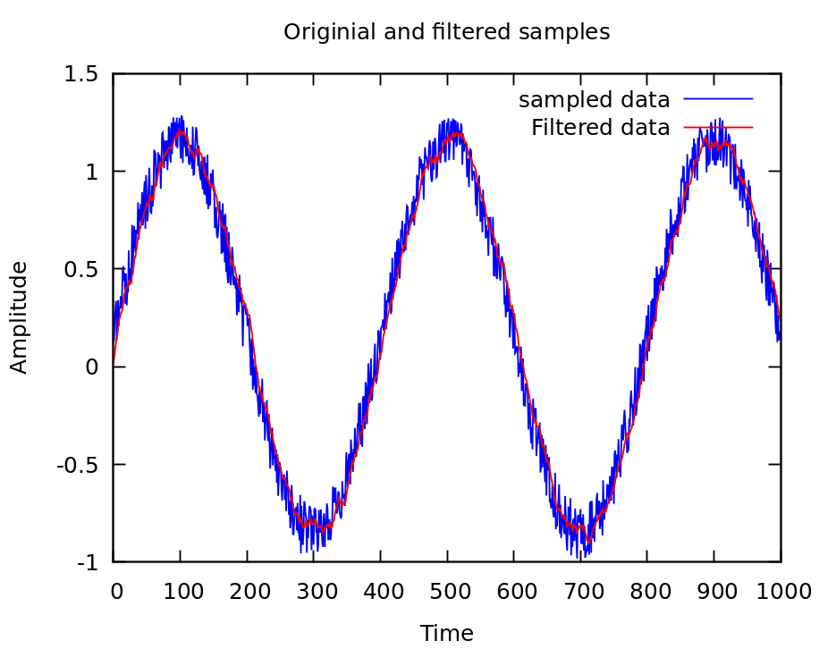
We can modify the impulse responds and filter length of the filter to have different filtering results. For example, we can set the filter length to 10 and the filter impulse responds as:
#define FIR_FILTER_LENGTH 10
and
static float FIR_FILTER_IMPULSE_RESPONSE[FIR_FILTER_LENGTH]={0.1,0.1,0.1,0.1,0.1,0.1,0.1,0.1,0.1,0.1};
The results of different filter length and impulse responds is show in figure 5. In figure 5, we can see that the filter has a more smoothing effect compared to the initial filter length and impulse respond.
Conclusion
In this post, we have shown a tutorial on how to implement a circular buffer concept for a FIR filtering application. In addition, we show how to visually plot the data with GNU plot using Linux piping operation.
The tutorial explains how to generate a noisy sinusoid signal, filter the signals and visually plot the results on a graph using GNU plot.
Also, the Linux compilation chain to compile the source codes into an executable file is also presented.
We sell all the source files, EXE file, include and LIB files as well as documentation of ellipse fitting by using C/C++, Qt framework, Eigen and OpenCV libraries in this link