Understanding measurement model, systematic error and random error

In this post, three important aspects in measurement are concisely discussed. The three aspects are measurement model, systematic error and random error.

These three aspects are essential for all measurements regardless the types of the measurements.

A measurement model (either a mathematical or empirical/statistical model) is important, especially if we want to apply GUM method to estimate the measurement uncertainty.

Measurement uncertainty is the quantification of random error estimation. Random error represents missing knowledge on a measurement process. That is, measurement uncertainty is the quantification of how unsure we are with regard to a measurement result.

Any systematic errors, commonly known as measurement bias, should be corrected before presenting any measurement results.

Next, we will discuss: measurement model, systematic error and random error.

Measurement model

In an ideal situation, a measurement result from a measuring instrument can be modelled as:

$y$=the instrument reading-the sum of all errors involved in the measurement

Where the sum of all errors involved in the measurement includes systematic (including calibration) errors and random errors.

This model in real situations is not applicable. Because, there are always errors that are unknown and should be quantified by uncertainty estimation.

In real situation the measurement model becomes:

$y$=the instrument reading - the sum of all known errors \pm the measurement uncertainty

So that the model is formulated as:

$y=x\pm U$

Where $x$ is the value of the instrument reading – all known (systematic) errors and $U$ is expanded uncertainty with 95% confidence interval.

According to VIM (BIPM 2008), error is the difference between the measured value and the true value of a measurement. Very often, the true value refers to a calibrated value (with valid measurement uncertainty statement).

There are two types of measurement error:

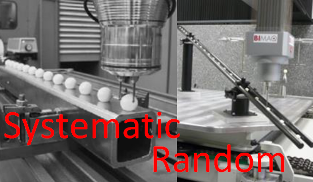
1. Systematic error
2. Random error

Hence the total error of a measurement is formulated as:

$total_error (\epsilon _{total})= systematic_error (\epsilon _{systematic}) + random_error (\epsilon _{random})$

Hence, the complete presentation of a measurement model is:

$y=x+\epsilon _{total}$

$y=x+\epsilon _{systematic}+\epsilon _{random}$

$(y-\epsilon _{systematic})=x+\epsilon _{random}$

$(y-\epsilon _{systematic})=x\pm U$

Where $U$ is expanded uncertainty with 95% confidence interval.

Systematic error

Systematic error is the deviation from the “true” value of a measurement that constantly repeats (re-occur) when the measurement is performed iteratively. In an easy word, systematic error is a repeatable deviation from the “true” value.

Note that the “true” value is in practice very often refers to a calibrated (reference) value.

Since systematic error has a re-occured pattern, systematic error can be modelled or estimated and then “off-line” compensated to increase the accuracy of a measurement result.

“Off-line” here means that the compensation method can be performed before a measurement results shown in an instrument or can be performed without a real-time feedback.

The compensation method for systematic error can be divided into two types: hardware compensation or software (numerical) compensation.

Hardware compensation is applied by adjusting or modifying components of an instrument to adjust the systematic error from the instrument. For example, by reducing the Abbe offset of the instrument or by reducing the angular error of the instrument linear axis.

Software compensation is applied by applying the model of a measurement in a software system and then corrected the reading of the measurement from an instrument. This compensation uses numerical calculation using the measurement model (either mathematical or statistical models) to correct the error from the measurement results.

Almost all modern measuring instruments implements software (numerical) error compensation to significantly increase the instrument accuracy with low cost.

Systematic error correction using hardware modifications or adjustments will significantly increase the instrument cost, compared to software compensation.

Random error

Random error is a measurement deviation that does not repeat when the measurement is performed iteratively. This error has no re-occurring pattern. Since there is no specific pattern that describes random error, random error cannot be “off-line” compensated.

Random error can only be quantified using statistics. The main quantification of random error is its statistical distribution along with the distribution’s parameters: mean and variance.

Random error can only be compensated “on-line”, meaning the compensation will require a real-time reading of actual measurement results and real-time feedback of the read measurement results to a closed-loop control system. The closed-loop control system will processed the feedback and adjust the result.

For example, in a linear motion stage, “on-line” compensation is performed as follow:

1. The linear stage is commanded to a specific position
2. The linear encoder in the stage read the actual position (different or deviated with the commanded position)
3. The actual position is sent back as feedback to a closed-loop control system.
4. This closed-loop control system compared the actual and commanded position and then calculate the required compensation
5. Then, the control system will add additional command to the linear stage to adjust the position to the commanded position based on the actual and commanded position difference

This online compensation is required since random error cannot be predicted (in term of its re-occurring pattern).

Since “on-line” compensation required more sensors, software and control electronics, implementing this type of control system will increase the cost of a measuring instrument.

However, this “on-line” compensation method can also compensate other non-linear high-degree errors (for example second-degree error) involved in a measurement process.

Commonly, “on-line” compensation method is implemented to achieve a very high accuracy of an instrument, for example sub-micrometre to nano-metre accuracy.

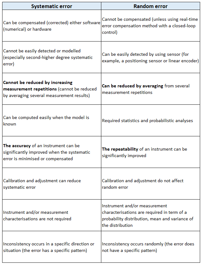
Table 1 shows the direct comparison between systematic and random error.

Conclusion

In this post, three aspects are discussed: measurement model, systematic error and random error. These three aspects are essential in any types of measurement.

By understanding the concept of measurement model, we can understand why we need to compensate systematic error (bias) in any measurement results and need to show the quantification of the remaining random error in term of statistical standard uncertainty.

Systematic and random errors are the two main types of error.

Systematic error is repeatable, can be mathematically modelled and can be “off-line” compensated.

Random error is non-repeatable, cannot be mathematically modelled, instead can only statistically quantified, and can only be “on-line” compensated.

We sell tutorials (containing PDF files, MATLAB scripts and CAD files) about 3D tolerance stack-up analysis based on statistical method (Monte-Carlo/MC Simulation).