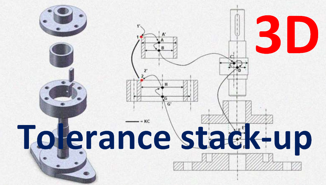
3D tolerance stack-up analysis with examples

In the previous post, tolerance stack-up analyses in 2D have been presented in detailed. However, the main disadvantage is that 2D tolerance analysis only predicts 2D on-plane variations and cannot predict rotational variations in 3D.

In this post, 3D tolerance stack-up analysis will be explained with two examples. Both traditional “+/-” dimensional tolerance and geometrical tolerance (GD&T) are considered.

The complete MATLAB implementations for the 3D tolerance analysis in this post can be obtained from here.

3D tolerance stack-up analysis

This tolerance analysis requires a matrix multiplication method to calculate the nominal and variation propagation on each part affecting the key characteristic (KC) of an assembled product.

With the matrix multiplication method, all linear and rotational errors of the KC of an assembly can be estimated in 3D with high accuracy (close to real-word situations).

We will discuss briefly some fundamentals related to the matrix multiplication method. Readers who are familiar with matrix concepts can skip this section and directly read the next section.

Homogenous matrix

Before discussing 3D tolerance analysis with the matrix method, the fundamental understanding of matrix should be obtained. The matrix type used for 3D tolerance analysis is homogenous matrix with size of $4\times 4$.

This homogenous matrix, that is as roto-translation matrix, will be used to represent roto-translation operations in 3D. With homogenous matrix, the roto-translation operations in 3D can be represented in a single matrix.

The format of a homogenous matrix is:

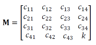
Where $c_{ij}$ is the $i$- and $j$-th element of the matrix and $k$ is a constant that is a scale of the matrix element $c_{ij}$.

In general, all $ c_{ij}$ and $k$ itself are divided by $k$ so that the scale $k$ value in the matrix becomes 1.

In 3D coordinate transformation calculations of a point P using homogenous matrix, the point P should also be represented in homogenous coordinate, that is:

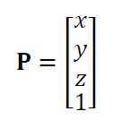
Where there is an additional 1 as the fourth element in the 3D position coordinate.

Roto-translational matrix

Before discussing roto-translation matrix, we will have a look at translation and rotation matrices individually.

A translation matrix Tr of a coordinate P is represented as:

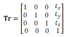
Where $t_{x}$ is a translation along x-axis, $t_{y}$ is a translation along y-axis and $t_{z}$ is a translation along z-axis.

Rotation matrices Rx, Ry and Rz that are rotation along x,y and z axes. These rotation matrices are represented as:

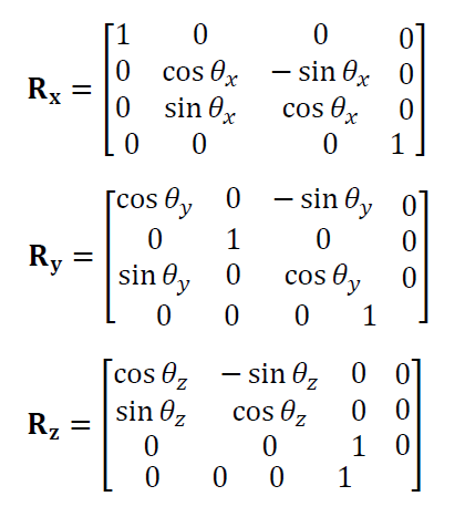
Where $\theta _{i}$ is rotation angle along i-axis.

Roto-translation matrix is a matrix that represents both translation and rotation transformations of a point with respect to an axis of rotation.

This roto-translation matrix is used to represent geometrical error variations of features on a part due to given or allocated feature tolerance values.

Very often, in the context of 3D tolerance analysis, a roto-translation matrix is called error matrix.

Error matrix

Error matrix is a roto-translation matrix Tij which has elements representing the value of translation or rotation variations of a feature due to allocated tolerances on that feature.

The error matrix Tij is represented as:

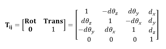
Where Rot is a $3\times 3$ matrix representing rotation error and Trans is $3\times 1$ column vector representing translation error. $d_{i}$ is the translation error component along i-axis in Trans column vector. $d\theta _{i}$ is the rotation error component along i-axis (in radian) in Rot matrix.

One thing to understand is that a roto-translation matrix first performs the translation of a point P and then performs the rotation to the point P.

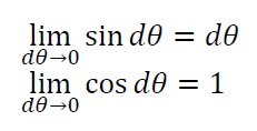
Note that the rotation errors in matrix Tij (elements of Rot) do not have $sin$ and $cos$. Because, errors elements in matrix Tij in general have very small values.

Hence, for a very small angle $\theta$ ($<0.3 rad$) the value of $sin(\theta )$ is close to the value of $\theta$ itself. And, the value of $cos(\theta )$ is close to 1.

The explanation of $sin$ and $cos$ approximations of very small angles is:

Coordinate transformation with matrix multiplication

It is important to understand the concept of matric multiplication to transform coordinates. In 3D tolerance stack-up analysis, symbol conventions to represent a point P and its transformation process are as follows:

• $P_{i}$ represents a point $P$ with respect to $i$ coordinate system
• $P_{j}$ represents a point P with respect to $j$ coordinate system
• $\mathbf{T_{ij}}$ represents a coordinate transformation from $i$ to $j$ coordinate system

The transformation is modelled as:

$P_{i}=\mathbf{T_{ij}} \cdot P_{j}$

The above equation is interpreted as follows. A point $P$, with respect to $i$ coordinate system, is the result of a transformation of the point $P$, with respect to $j$ coordinate system, by using a transformation matrix $\mathbf{T_{ij}}$.

To reverse the operation, that is obtaining the point P with respect to $j$ coordinate system, $P_{j}$, the transformation is:

$P_{j}=\mathbf{T_{ij}^{-1}} \cdot P_{i}$

Where $\mathbf{T_{ij}^{-1}} =\mathbf{T_{ji}}$.

To ease the naming convention in variation transformation chains (discussed in the next section), the index of the matrix can be written as:

$\mathbf{T_{ii’}}$

Representing a transformation from a nominal point $i$ to a deviated point $i’$ on a feature due to dimensional and geometrical variations.

Figure 1 shows a pictorial presentation of coordinate transformation. From figure 1, an intuitive understanding can be obtained for coordinate transformation to get a point P with respect to coordinate system 1 from point P with respect to coordinate system 2.

Nominal and variation transformation chains

Before performing 3D tolerance analysis, the model of nominal and variation transformation chains of an assembly should be obtained.

Figure 2 represents the nominal and variation tolerance chains of an assembly to be analysed. In figure 2 left, a nominal tolerance chain follows the nominal dimension of all features passed by the tolerance chain of an assembly.

Meanwhile, figure 2 right shows additional transformations added to the nominal chain due to variations on the features obtained by allocated tolerances.

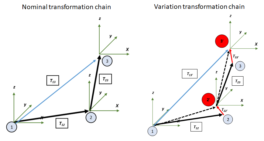
In figure 2 right, matrix $\mathbf{T_{12}}$ transforms the coordinate system 1 (on a feature 1) to the coordinate system 2 (on a feature 2) and matrix $\mathbf{T_{23}}$ transforms the coordinate system 2 (on a feature 2) to the coordinate system 3 (on a feature 3).

Because there is a variation on feature 2 (represented by the type and value of a tolerance assigned to this feature), there are an additional transformation describing the variation on feature 2, that are $\mathbf{T_{22’}}$ due to variations on feature 2 and $\mathbf{T_{33’}}$ due to variations on feature 3.

Example 1: 3D tolerance stack-up analysis of two parts with GD&T

This example uses the same two-part assembly as in the previous example of 2D tolerance analysis (including the parts and assembly detailed drawings for the nominal dimensions and tolerances in this example).

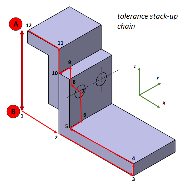
Figure 3 shows the tolerance chain and the key characteristics (KC) of the assembly. The KC is the distance and orientation variations between point A and B. In figure 3, the tolerance chain is in 3D.

the tolerance chain should pass the assembly features of the two parts. The assembly features are the features that connect the two parts.

The selection of tolerance chain should represent as close as possible on how the assembly will function.

Nominal transformation chain

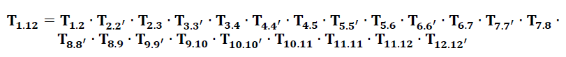
From the tolerance chain (figure 3), the nominal transformation chain of the assembly is:

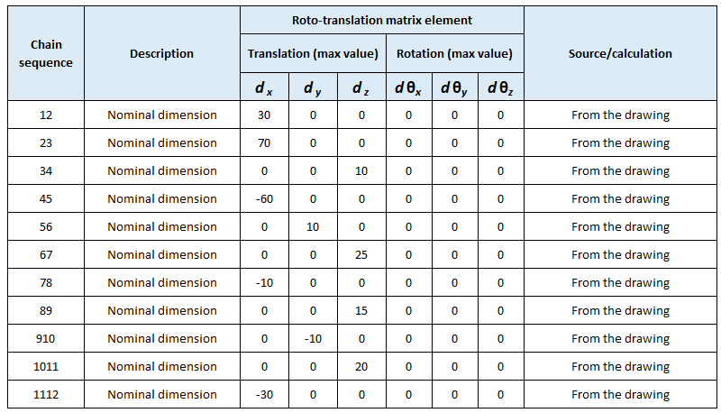
Where each $\mathbf{T_{ij}}$ contain elements: $d_{x}, d_{y}, d_{z},d\theta _{x}, d\theta _{y}, d\theta _{z}$ that represent variation due to allocated tolerances. $\mathbf{T_{1.12}}$ is the total variation from point 1 to point 12 in the tolerance chain.

The values for all $d_{x}, d_{y}, d_{z},d\theta _{x}, d\theta _{y}, d\theta _{z}$ elements on each transformation matrix $\mathbf{T_{ij}}$ are presented in table 1. In table 1, each row represents a transformation from point $k$ to point $k+1$ in the tolerance chain.

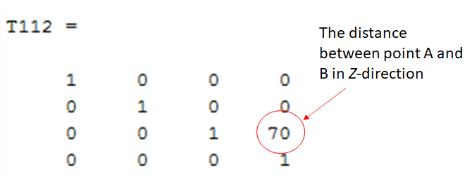
After establishing the nominal transformation chains and the elements of transformation matrices in the nominal chain, the nominal distance between A and B can be calculated by multiplying all the $4\times 4$ matrices in the nominal transformationchain. The results of the multiplication is the matrix $\mathbf{T_{1.12}}$ .

The result of matrix $\mathbf{T_{1.12}}$ is shown in figure 4. In figure 4, the nominal distance from A to B (the KC) is $70 mm$ in $z$-direction.

This value is obtained from the (3,4)-element of matrix $\mathbf{T_{1.12}}$. The elements of (1,4) and (2,4) are the nominal distance between point A and B in $x$ and $y$ direction and are zero.

And, the elements of (1,2), (1,3), (2,1), (2,3), (3,1) and (3,2) of matrix $\mathbf{T_{1.12}}$ are the rotational variations between point A and B along $x,y,z$-axes. As can bee observed, in perfect condition, there will be only a translation from A to B in $z$-direction for $70 mm$ and there are no rotations.

The calculation of nominal transformation chain is useful to verify whether our designed KC (in this example the distance between A and B) is correct in case of perfect condition.

Variation transformation chain

The next step is to establish the variation transformation chain from the tolerance chain (figure 3). The variation transformation chain is:

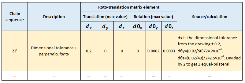
An example on how to calculate the elements $d_{x}, d_{y}, d_{z}, d\theta _{x}, d\theta _{y}, d\theta _{z}$ of the variation matrices $\mathbf{T_{ij’}}$ involved in the variation chain is shown in table 2 below. Note that, all elements for the nominal matrix $\mathbf{T_{ij}}$ are the same as before.

The detailed calculations of each variation in the tolerance chain for example 1 can be obtained from here.

In table 2, every row of nominal chain is followed by a row of its variation chain. All rotational variation elements $d\theta _{x}, d\theta _{y}, d\theta _{z}$ are in radian.

Note that for the variation matrices $\mathbf{T_{ij’}}$, elements $d_{x}, d_{y}, d_{z}$ are commonly from the dimensional tolerances assigned to features and bonus tolerances, from the allocated GD&T tolerances.

Meanwhile, elements $d\theta _{x}, d\theta _{y}, d\theta _{z}$ need to be calculated and are related to the dimension of the features and allocated GD&T tolerances as well.

The explanations to calculate the values of elements $d\theta _{x}, d\theta _{y}, d\theta _{z}$ are as follow.

In principle, the values of $d\theta _{x}, d\theta _{y}, d\theta _{z}$ follow the largest values of the tolerance zones of geometric tolerances on features (that is a worst-case assumption on the geometric tolerances). The tolerance zones can be a cylinder or two-parallel planes.

For the tolerance zone in the form of two-parallel planes (figure 5 top), the value of $ d\theta _{i}$ $ is calculated by the value of tolerance zones divided by the length (or width) of the surface of a feature.

For the tolerance zone in the form of a cylinder (figure 5 bottom), the value of $ d\theta _{i}$ $ is calculated by the value of tolerance zones divided by the height of a cylindrical feature (representing the feature or the height of the cylinder tolerance zone).

Note that to follow the equal-bilateral format, the calculated $ d\theta _{i}$ is, then, divided by 2.

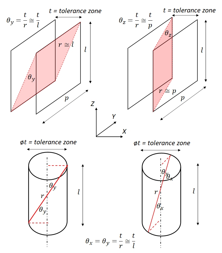
Note that from figure 5, to calculate the $d\theta _{x}, d\theta _{y}, d\theta _{z}$, one thing to remember is that rotational errors will have relatively large values if the height of hole features is made short or the area of plane features is made small. Because, mathematically, de-numerators to calculate the angular errors become small and then the value of the angular errors become large.

The physical interpretations are that when a hole feature, usually where a pin will be inserted, is made short the pin-hole join will be not stable. Similar to a surface, if the surface area of plane features is made small, the surfaces become unstable and the manufacturing variations (used to make the surface) become high.

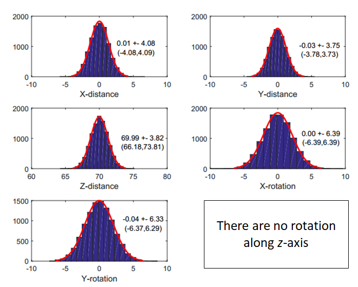
The 3D tolerance stack-up analysis is based on statistical method. A Monte-Carlo (MC) simulation is used to re-calculate the total variation transformation chain (the final variation matrix) for a large number of times.

On each simulation run, we sample each element of $d_{x}, d_{y}, d_{z}, d\theta _{x}, d\theta _{y}, d\theta _{z}$. The samples are generated from normal distributions with mean 0 and standard deviation $\sigma$ equal to the error elements divided by 2, that are $N~(0,\sigma ^{2})$ where $\sigma=\frac{d_{i}}{3}$ and $\sigma=\frac{d\theta _{i}}{3}$.

Figure 6 shows the results of the total variation of the distance and orientation between point A and B after 10000 simulation runs. From the results, the distance between point A and B in $z$-direction is $(69.99\pm 3.82)mm$ or $66.18-73.81$. Note that in figure 6, there is no rotation a long $z$-axis as this rotation will not have any effect to point A and B in term of distance and rotation.

All detailed calculations of each variation matrix and the MATLAB codes implementations to run the MC simulation can be obtained from here.

Example 2: 3D tolerance stack-up analysis of a rotary compressor with GD&T

In this example, not only 3D tolerance analysis will be explained, but also other aspects: tolerance allocation, design revision and tolerance re-allocation will be discussed.

The rotary compressor is a type of air compressor to provide high pressure air. The working principle of a rotary compressor is that a cylindrical rotor rotates inside a cylindrical cavity with bigger diameter with the rotor. The axis of the rotor and the cavity is not coaxial.

With this non-coaxial axis configuration, two asymmetric volumes are created when the rotor rotates and causes a working pump effect. In the intake part of the cavity, the volume increases when the pump in operation. Meanwhile, in the outtake part, the volume of the cavity decreases.

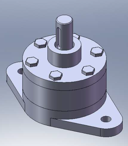
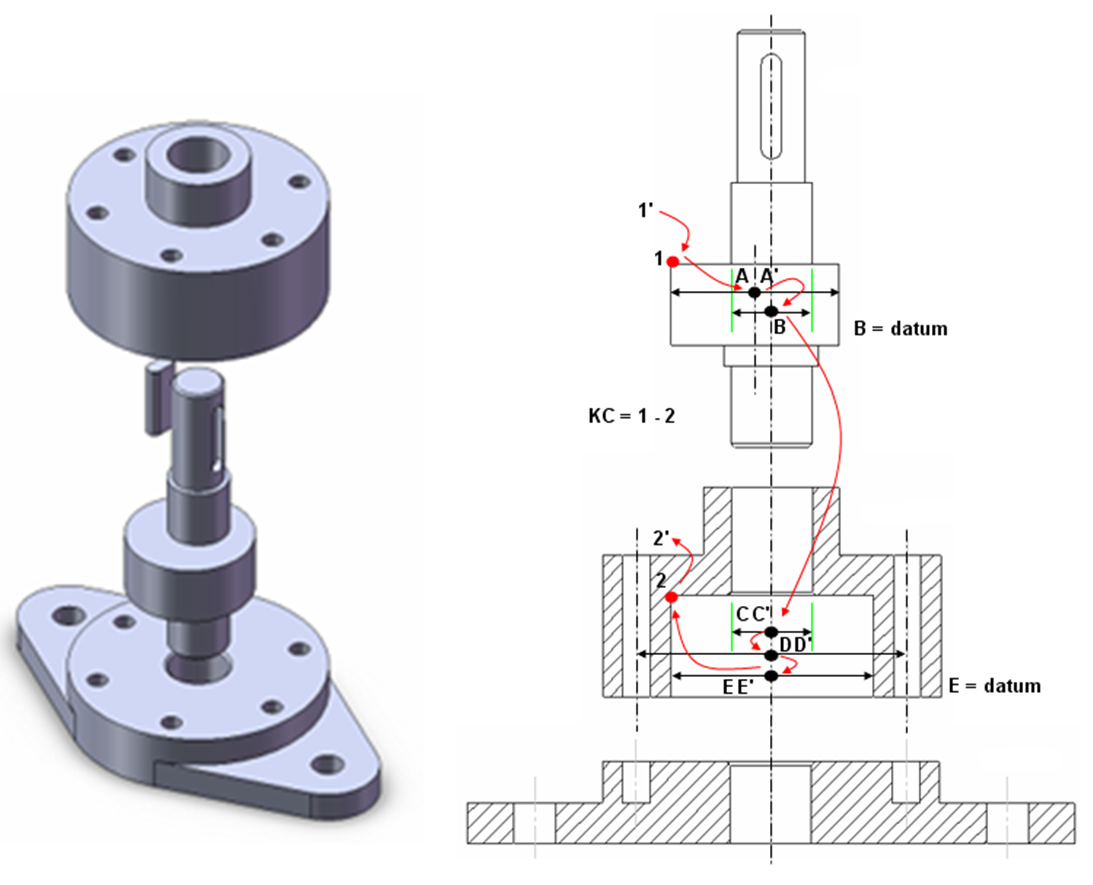
Rotary compressors are commonly found as high-pressure hydraulic pump, such as transmission pump in a car, power-steering pump and vacuum pump. Figure 7 shows the assembly of the rotary compressor. The main components of the compressor are a rotor, shaft, body, base and cover.

In this example, two types of design of the compressor are presented: initial design and revised design. Brief explanations about the tolerance analysis and allocation in both designs are presented.

Meanwhile detailed tolerance analysis calculations re-design processes and MC simulation of the analysis can be obtained from here.

Initial design and the tolerance analysis

The initial design consists of five main parts: base, body, rotor, poros (shaft) and cover. Figure 8 shows the detailed drawing of the five parts constituting the rotary compressor based on the initial design. In figure 8, both traditional “+/-” dimensional and GD&T tolerances are used.

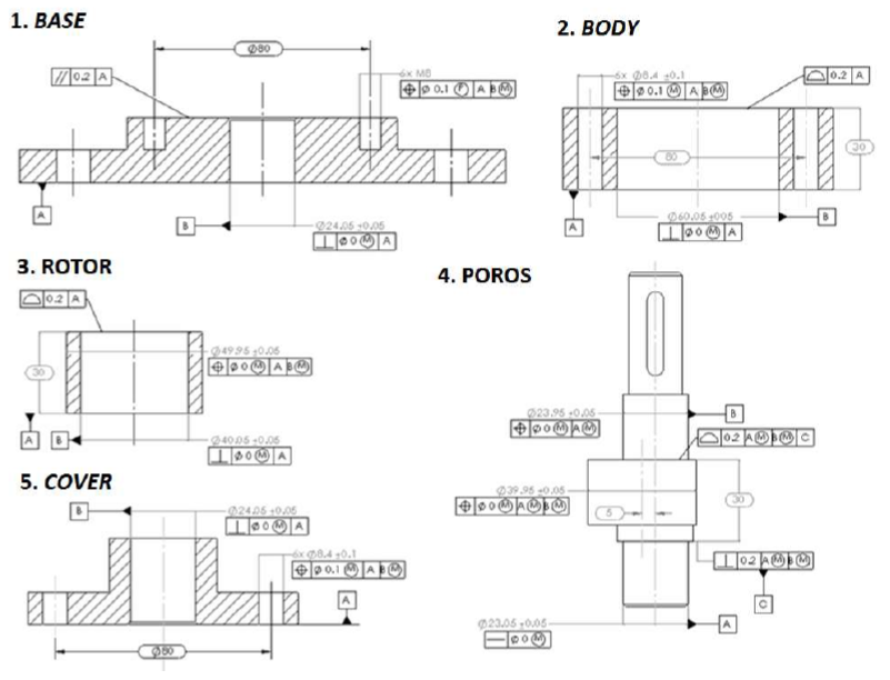
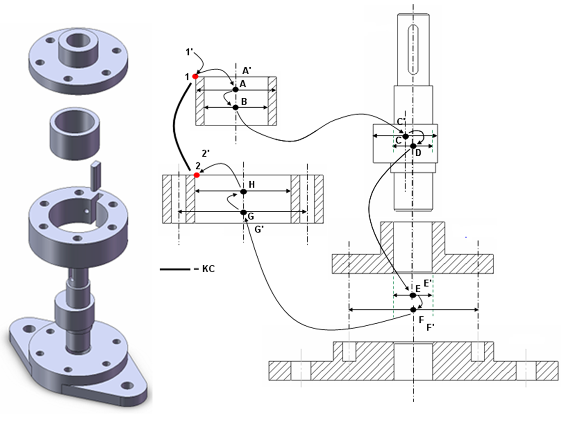
Figure 9 shows the initial design of the components of the compressor and the tolerance chain of the compressor assembly.

The KC of the assembly is the distance between point 1 and 2 that should be between $0mm-0.5mm$. If there is an interference between point 1 and 2, then, there will be frictions between the rotor and shaft (to create the asymmetric cavity) and cause significant wear of the compressor while operating. Meanwhile, if the gap is too big, then the compression performance will be significantly reduced.

From the tolerance chain shown in figure 9, the nominal and variation transformation chains are constructed and calculated. MC simulations are performed for 10000 runs.

Tolerance allocation to determine the values of all error elements in the variation matrices have been optimised before running the simulation. The results of total variation matrix calculated on each run are stored and statistically analysed.

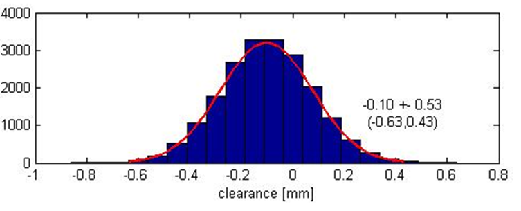
Figure 10 shows the results of the MC simulations. From MC simulations for the 3D tolerance analysis of the initial design, the distance between point 1 and 2 is ($-0.1\pm 0.53mm$) or $-0.63mm-0.43mm$.

From figure 10, even after tolerance re-allocation optimisation, with the initial design the desired KC, that is the distance between point 1 and 2 to be $0mm-0.5mm$, cannot be achieved. Hence, a redesign process of the compressor need to be carried out.

Revised design and the tolerance analysis

The redesigned or revised compressor has reduced parts to be only three parts: base, cover+body and poros (shaft)+rotor. Figure 11 shows the parts for the redesigned compressor.

Note that there are two parts that are joined parts. With the reduced parts, the number of variations in the variation propagation chain (tolerance chain) is reduced and then the total variation stack-up is also reduced.

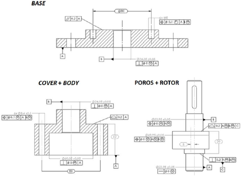
Figure 12 shows the tolerance chain of the revised designed. Similar to the initial design, the KC is the distance between point 1 and 2 so that there is no interference between point 1 and 2 to avoid frictions during operation.

The nominal and variation transformation chain can then be derived from the tolerance chain in figure 12. Also, the MC simulations are performed for 10000 runs as applied to the tolerance analysis for the initial design.

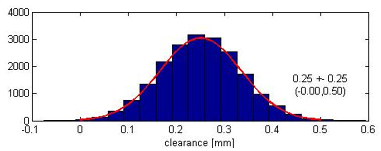
Tolerance allocation before running the MC simulations has also been optimised. Figure 13 shows the results of the MC simulations for the revised design.

From the simulations, the estimated distance variation between point 1 and 2 is ($0.25\pm 0.25mm$) or $0.0mm-0.5mm$.

Form this result, the desired KC can be achieved by revising the initial design and perform the optimisation of tolerance re-allocation to the parts on the revised design.

The detailed calculations of each variation in the tolerance chain, tolerance allocation and re-allocation, redesign processes and the MATLAB code to run MC simulation for example 2 can be obtained from here.

Conclusion

This post presents tolerance stack-up analysis in 3D with examples: a two-part assembly of prismatic product and a rotary-compressor. Both “+/-” dimensional tolerance and geometrical tolerance (GD&T) are considered.

In 3D tolerance analysis, a $4\times 4$ homogenous transformation matrix is used to calculate the propagation of variations on each part constituting an assembly.

The main advantage of 3D tolerance analysis is that assembly variations can be calculated in 3D space including rotational variations.

With 3D tolerance stack up analysis, the variation of an assembly can be predicted more accurate than 2D tolerance stack-up analysis.

The detailed calculations of each variation on the tolerance chains and the MATLAB codes for the simulation in the example 1 and example 2 can be obtained from here.

If you think this article is useful and want to support me developing this blog, you can support me here.