2D tolerance stack-up analysis with examples

Every part constituting an assembled product has tolerances assigned to the part’s features. These assigned tolerances cause variations on the key characteristics (KCs) of the assembled part.

How can we know how much the variations on the KCs before manufacturing the parts?

This post will explain the method used to analyse tolerance/variation stack-ups in 2D. Examples are given to give a clear understanding on how to perform 2D tolerance stack-up analysis on parts.

(You may read a post about the explanation of assembly and key characteristic)

for 3D tolerance stack-up analysis, you can read here.

Tolerance stack-up analysis

Tolerance stack-up analysis is a method used to evaluate the cumulative effect of tolerances allocated on the features of components and to assure that the cumulative effect is acceptable to guarantee the functionality of a product after assembly processes (see this book).

Different names refer to the same tolerance stack-up analysis, such as: tolerance analysis, tolerance-chain analysis, variation stack-up analysis and assembly-chain analysis.

The main goal of tolerance analysis is to check that the dimensions and tolerances of components are correct so that after the components are assembled, the assembled product can function as desired.

Tolerance stack-up analysis is unique because this analysis is half-science and half-art (depends on how we determine a tolerance chain)

Tolerance allocation and tolerance stack-up analysis always come “hand-in-hand” and cannot be separated each other. Tolerance stack-up analysis and tolerance allocation are iterative processes that are carried out until the desired KC of an assembly is satisfied based on given geometrical and dimensional tolerances (GD&T) on parts.

A systematic approach on tolerance stack-up analysis is necessary to reduce the number of iteration processes to determine correct tolerance values on part’s features.

The experience of design and manufacturing engineers play an important role on the first determination of tolerance values. Because, the value of tolerances are directly related to how difficult a part can be made and how much the cost to make the part.

The smaller the tolerance value, the tighter the tolerance, and then the higher the production and inspection cost, and otherwise.

Questions to be answered by performing tolerance stack-up analysis

By performing tolerance stack-up analysis, important questions regarding the assembly process and the final KC of a product can be answered before manufacturing, for examples:

• What is the effect on a final assembled product when the location of a hole on a bracket deviating few millimetres from the hole nominal position?
• How much material need to be preserved in a machining process so that there are still materials for post-processing, for example boring process, to get smooth surface finish or high dimensional accuracy on a feature?
• What is the effect if a manufactured hole is made larger from its nominal diameter?
• What is the effect if the number of components constituting an assembly are added?
• Does the surface of the rotor and stator of a motor touch each other during operation?
• How much the gap or clearance variation between two surfaces of a part after an assembly process?
• How much the optimal temperature of the assembly process of a micro-scale product should be to eliminate or reduce the effect of component thermal expansions during the assembly process so that the KC of the product can be maintained?

General steps or procedures to perform tolerance stack-up analysis

1. Define the critical dimension (KC) of the assembly feature of a product to be analysed, such as clearance between two plates
2. Construct the tolerance chain of the product, that is the chain of components that affect the assembly feature or critical dimensions
3. Define the model of the tolerance stack-up
4. Consider all possible variation sources on the model
5. Add all the variation sources, either with worst-case or statistical based methods (see the following section).

Tolerance analysis methods: worst-case and statistical based

In general, there are two types of methods to add all variations in tolerance stack-up analysis, that are:

Worst-case based analysis

Worst-case analysis is a tolerance analysis method that adds all maximum values of allocated tolerances. Worst-case analysis is formulated as:

Total variation = $Tol_{1}+ Tol_{2}+ Tol_{3}+ … + Tol_{n}=\Sigma_{i=1..n}Tol_{i}$

Where $ Tol_{i}$ is the $i$-the tolerance in equal-bilateralformat ($\pm Tol_{i}$).

The properties of worst-case based analysis are:

• This method represents the largest possible variation on an assembled product based on allocated tolerance values
• This method assumes that all components are in their largest deviation at the same time in assembly processes (in reality, this situation rarely happens as very often, one feature deviate at maximum and the other features are not)
• This method requires all parts should be inspected one-by-one to assure that there is no single part that is out of tolerance.
• This method is suitable for low-volume and high-value products such as jet engines that need inspection for each engine.
• This method implies that when all parts constituting an assembly are in conformance then the assembly (KC) will be assured to be in tolerance.

Statistical based analysis

Statistical-based analysis is a tolerance analysis method that sum-of-squares all values of allocated tolerances. This method assumes some degree of confidences on the estimated sum-of-squares total variations ($2\sigma$ is 95% confidence).

The formula for statistical-based analysis is:

Total variation = $k\sqrt{ Tol_{1} ^{2}+ Tol_{2}^{2}+ Tol_{3}^{2}+ … + Tol_{n}^{2}}=k\sqrt{\Sigma_{i=1..n}Tol_{i}^{2}}$

Where $ Tol_{i}$ is the $i$-the tolerance in equal-bilateralformat ($\pm Tol_{i}$) and $k$ is a safety factor to take into account variances from components supplied from other companies. In general, $k=1.5$ if components are supplied from other companies. If all components are made in-house, $k$ can be set to 1 (meaning the variations of components can be controlled because the components are made in-house).

The properties of statistical based analysis are:

• This method requires the production processes of products to be analyses are in control, that is operating under the process normal condition. To determine whether a process is in or out of control, process capability index calculations can be performed ($C_{p}>1$)
• This method requires there is no mean-shift on the production processes of products ($C_{pk}>1$)
• This method assumes that all dimensions of features are very likely to be at their nominal values because the production processes of the features are controlled
• This method will have total variation values to be less than the values calculated based-on worst-case method. This lower variation values mean that the values for allocated tolerance on features can be made larger (than that when using worst-case method) so that the production and inspection cost can be reduced
• This method assumes that inspection processes are not performed for all parts. Instead, the inspection processes are performed to some products in a batch by random sampling
• This method implies that when all parts constituting an assembly are in conformance then there will be low probability that an assembly (KC) is out of tolerance.

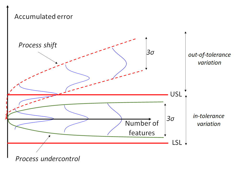
Figure 1 shows an illustration of the effect of mean-shift of the production process of a component. In this illustration, even if the process is under control (the process variations on both red and green situations are within $3\sigma$ tolerances), the produced component will be out of its tolerance.

EXAMPLE 1: 2D tolerance analysis with “+/-” tolerance

In this example, the slot feature of a component made by a milling process is analysed. Figure 2 shows the dimensions and tolerances of the features on the component. The KC is the distance between the two slots.

In figure 2, the tolerance is shown in two formats: unequal bilateral (figure 2 left) and equal bilateral (figure 2 right) formats. Both worst-case and statistical-based analyses require tolerances to be in equal bilateral format.

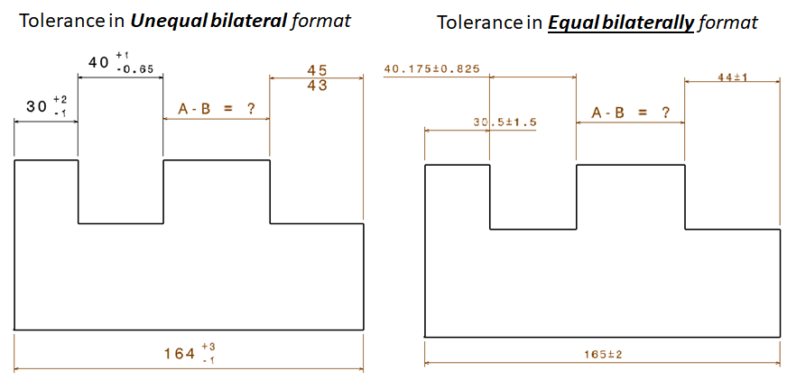
The format of equal bilateral tolerance is

$X\pm T$

Where $X$ is nominal dimension and $T$ is tolerance of “X”.

To convert the format of tolerances from unequal bilateral to equal bilateral, the following procedure is used:

$X=\frac{min+max}{2}$

$T=\frac{min-max}{2}$

Where $min$ and $max$ are the minimum and maximum value, respectively, of a dimension and tolerance.

To perform the tolerance stack-up analysis, we need to define the tolerance chain of the part. Figure 3 shows the KC and tolerance chain of the part in figure 2. Tolerance chain describes the propagation of accumulated tolerances from point A to point B.

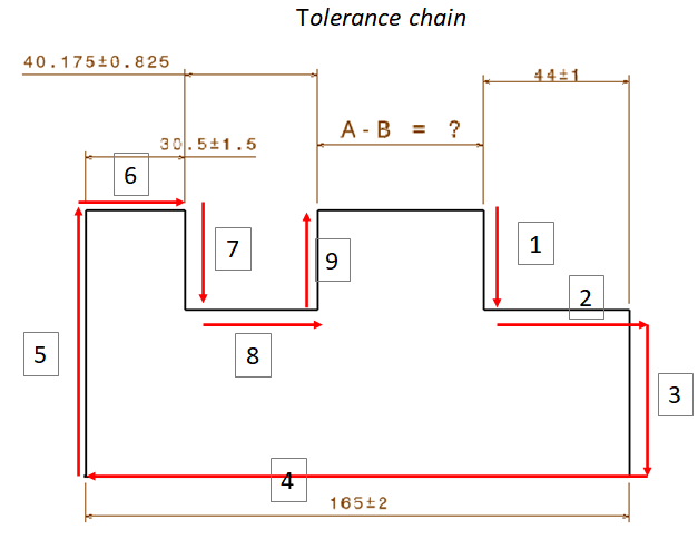
From figure 3, we can perform the tolerance analysis with both worst-case and statistical-based methods.

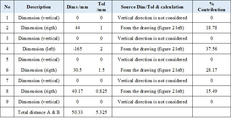
Table 1 shows the analysis based on worst-case method. The direction of tolerance propagations that are relevant is only in horisontal direction. From table 1, the results of the total variation based on worst-case method is that the distance variation between point A and B is $5.325mm$ and the nominal distance is $50.33mm$.

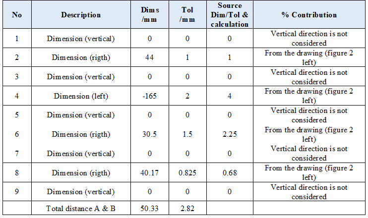
Meanwhile, table 2 shows the analysis based on statistical method. From table 2, the total variation calculated by statistical-based method is $2.82mm$ with the same nominal dimension of $50.33mm$.

As explained before, with statistical-based method, the total variation is smaller than that calculated from worst-case method. In this case, the total variation calculated by using statistical-based method is 47% lower than that of worst-case method.

This smaller total variation implies that with statistical-based method, we can allocate higher values for the tolerance than with worst-case method. This higher tolerance values mean that the part can be manufactured and inspected at lower cost than the one with tighter tolerance.

EXAMPLE 2: 2D tolerance analysis with GD&T tolerance

In this example, an assembly consisting of two parts is used. The assembly use not only “+/-” tolerance, but also geometric tolerance (GD&T).

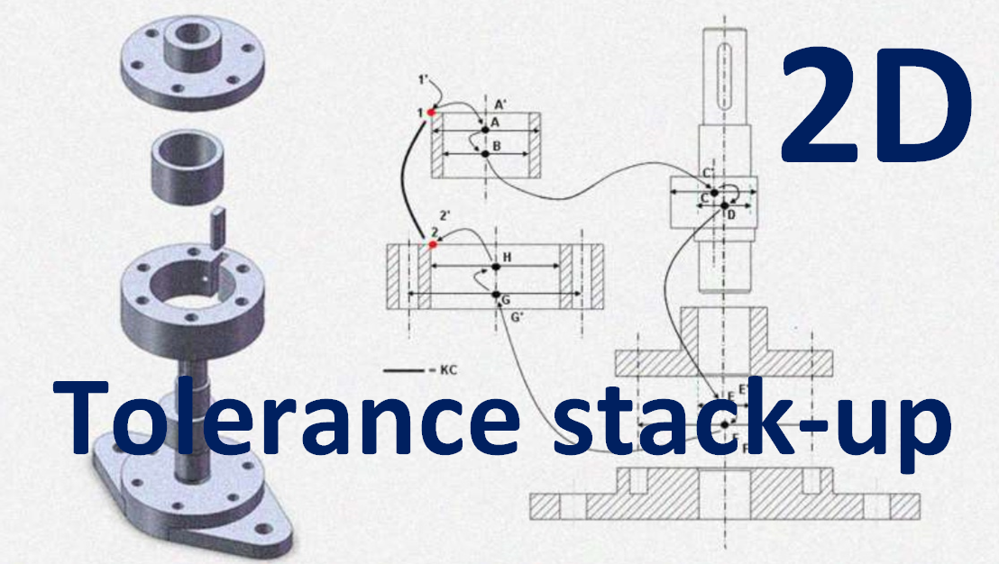
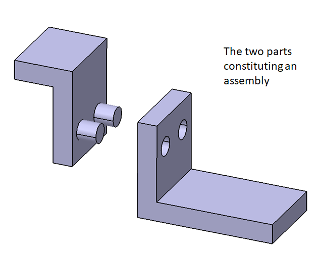
Figure 4 shows the two parts used in this example. The assembly features are the two pins and holes of the parts. These pins and holes are the features that join the two parts.

It is worth to note that, in general, with additional geometric tolerances, the total variation will be higher than in the case where only “+/-” tolerancing is used. The reason is that with geometric tolerance, the source of tolerance values is more than only use “+/-” tolerances.

However, with GD&T, the tolerancing of the part is better than only using “+/-“ tolerances. Because, with GD&T, the representation of the parts and assembly considers the real conditions of the manufacturing process of the parts so that the results of the tolerance analysis will be significantly more accurate than the analysis that only considers “+/-” tolerance (you may read this post for more explanations).

The detailed dimensions and tolerances of the two parts are shown in figure 5 and 6. It is worth to note that in figure 5 and 6 there are datums. These datums are the requirements of using GD&T, especially to tolerance related features.

In figure 5, datum A (the most stable and easy to access surface on a part) on part 1 is the top surface of the part and is given a flatness tolerance, that is an unrelated tolerance (the family of form tolerance).

Datum B and C are assigned to the side surfaces of datum A and are given perpendicularity tolerances with respect to datum A. All geometrical tolerances on this part will refer to these datum A,B and/or C.

In figure 6, datum A (again, the most stable and easy to access surface on a part) on part 2 is the bottom surface of the part and is also given a flatness tolerance. And, similar to part 1, the other datum B and C are assigned to the side surfaces of datum A.

It is important to note that datum A on both part 1 and 2 has the smallest (tightest) tolerance values compare to other tolerances. The reason is that datum A is the main reference of other datums and tolerances and should be manufactured with the highest accuracy compared to other features on part 1 and 2.

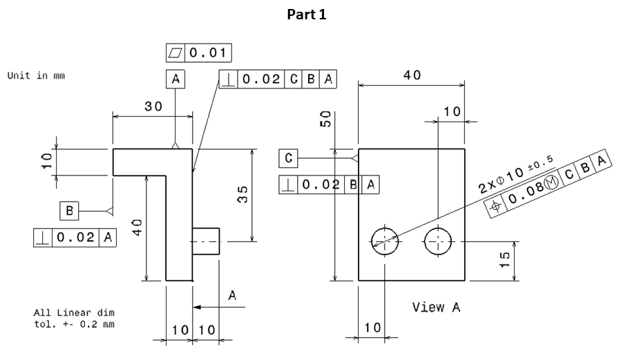
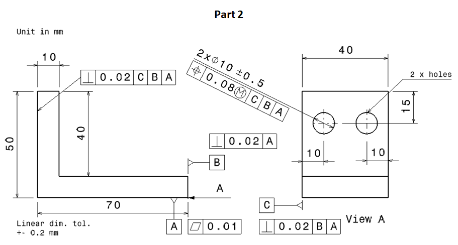
In figure 5 and 6, to tolerance pin and hole features, position tolerances are commonly used. The reason is that position tolerance also controls cylindricity of the pins and holes.

Figure 7 shows the tolerance chain of the two parts’ assembly. The KC is the vertical distance between point A and point B and also shown in figure 7. In figure 7, we can observe there are many variation sources related to the centre of the pins and holes that are the assembly features.

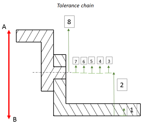
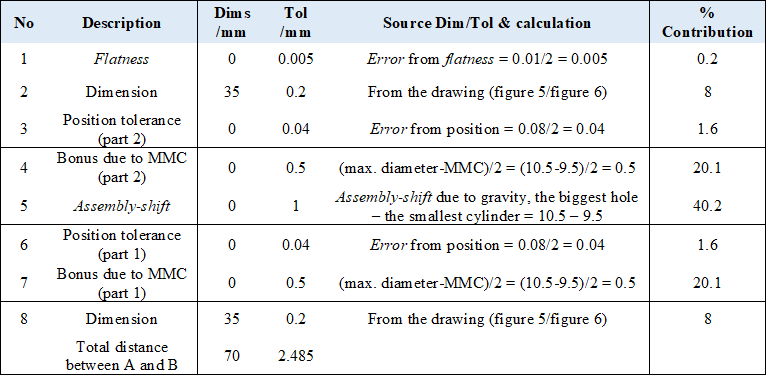
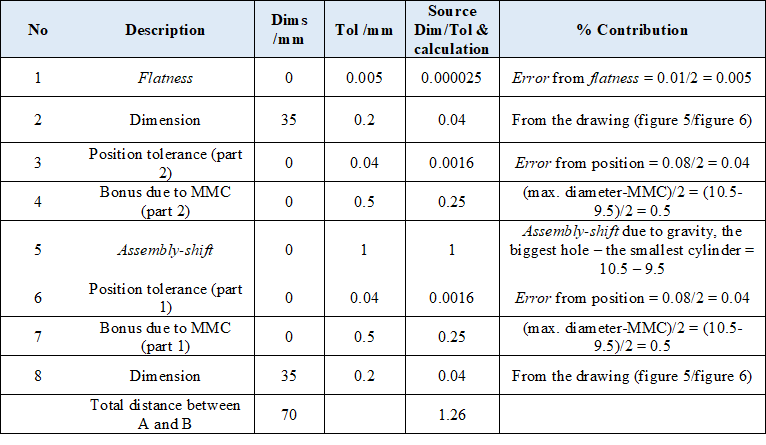
Table 3 shows the results of the 2D tolerance stack-up analysis based on worst-case method and table 3 shows the results of the analysis based on statistical method. As can be observed from table 3 and 4, beside assembly shift, other variations occur and are caused by bonus tolerances.

These bonus tolerances are obtained because the hole and pin features deviates from the maximum material condition (MMC) of the holes and pins.

The results of the tolerance analyses with the two methods are $(70\pm 2.485) mm$ for the calculation based on worst-case method and $(70\pm 1.26) mm$ for the calculation based on statistical method.

EXAMPLE 3: 2D tolerance analysis of a real product with GD&T tolerance

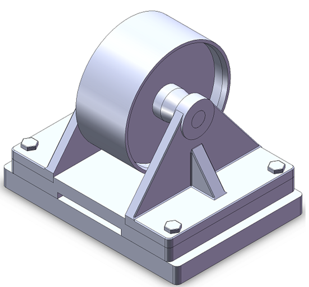
A belt-tensioner assembly is presented in this example. The belt-tensioner has a function to provide force so that the tension level of a belt can be maintained.

Belt-tensioners are commonly found on various applications, such as timing-belt systems in car engines, chain tensioners in bicycles and conveyor belts in factories. The main components of a belt-tensioner are pulleys to bear the belts so that tensions can be applied to the belts.

The distance between the pulleys and the base on the tensioner should be maintained. Because, the pulley should not touch the base when the tensioner is in operation.

In this example, both tolerance analysis and allocation will be presented. The 2D tolerance analyses of the parts constituting the belt-tensioner assembly use both worst-case and statistical-based methods.

The design of the belt-tensioner

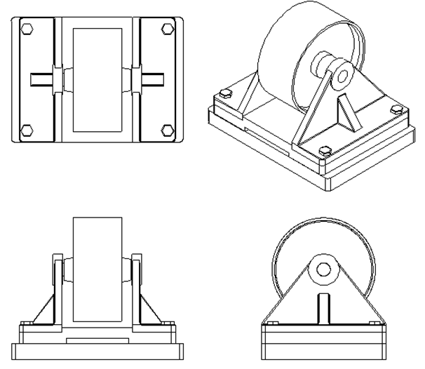
The design and assembly of the belt tensioner are shown in figure 8. Meanwhile, figure 9 shows the different 2D projection views of the belt-tensioner assembly.

There are four main parts constituting the assembly: base, support, rotor and pulley. The KC or the assembly key characteristic that should be controlled is the clearance between the pulley and the base so that there is no friction between the pulley and base during operation.

The nominal dimension and tolerances (both “+/- ” and GD&T) of the parts are shown in figure 10. In figure 10, for the base, there are three datums: A, B and C. Datum A (selected due to the surface is the most stable and easy to access) is the main reference and has a flatness tolerance of $0.01 mm$, that is the tightest tolerance due to datum A is the main reference for all geometric tolerances on the base.

The other geometric tolerances on base are profile tolerance and position tolerance. The position tolerance controls the accuracy of the holes as the features to assemble other parts to the base.

For the support (figure 10), the most stable surface for datum A is the bottom surface of the support with flatness tolerance of $0.01 mm$. The other datums are datum B and C that have perpendicularity tolerances with respect to datum A.

The datum B and C on the support is used as the references of the hole position to insert the rotor part. Other geometrical tolerances on the support are profile tolerances to control the surface profile of the surfaces.

For the rotor (figure 10), the most stable feature for datum A is the main axis of the cylinder. Because, the rotor is cylindrical and does not have a large stable or flat surface. Geometric tolerances applied to the rotor are cylindricity to control the cylinder shape including the axis and position tolerances to control the axis of the middle cylinder.

Finally, the dimension and tolerance for the pulley (figure 10) are similar to the rotor part as both the pulley and rotor are cylindrical parts. Datum A is the internal (middle) cylinder of the pulley. Position tolerances are applied to control the axis of the big cylinder to be coaxes with the middle cylinder (datum A).

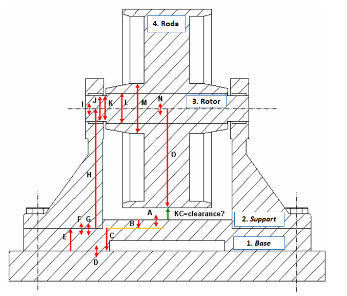
Tolerance chain of the belt-tensioner

The tolerance chain of the belt-tensioner is shown in figure 11. In figure 11, the KC is clearance or gap between the pulley and base, as being mentioned above, and is shown as green arrow in figure 11.

Since the analysis is 2D, we only consider variation in horizontal and vertical directions. Specifically for this case, only variation chains in vertical direction are relevant since the clearance (KC) is in vertical direction.

The tolerance chain is shown as red arrows and is flowing through the features affecting the KC. The determination of this tolerance chain is half-science and half-art. Because, very often, there are several ways in defining the tolerance chain of an assembly.

Tolerance analysis and allocation

From figure 11, the tolerance chain is A—B—C—D—E—F—G—H—I—J—K—L—M—N—O. B,C,E,H are nominal dimensions so that their variations are zero. A,D,F,G,I,J,K,L,M,N,O are due to tolerances both dimensional and geometrical tolerances so that the mean value is zero.

Table 5 shows the detailed calculation of the mean ($X_{n}$) and variation ($T_{x}$) for each point on the tolerance chain in figure 11. In table 5, the mean and variation value for each point on the chain are presented. Note that the tolerance format is in equal-bilateral format.

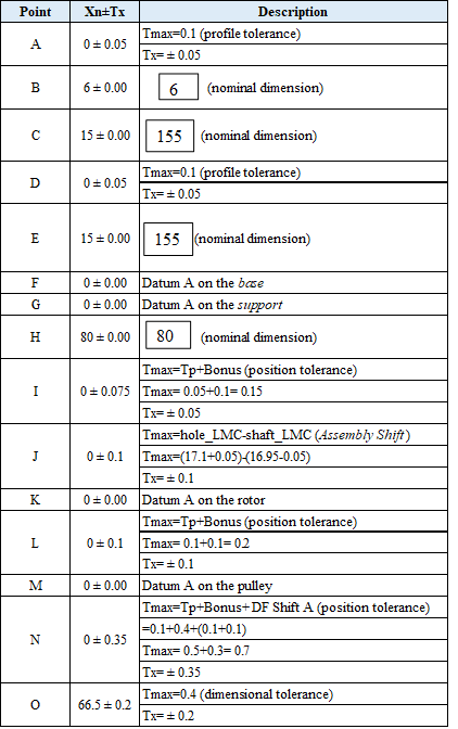
As can be seen in table 5, the nominal values ($X_{n}$) for all geometrical tolerances (at point A, D,F,G, I,J,K,L,M,N) are always zero. Because, in perfect condition, all geometrical variations should be zero.

The nominal value of the KC (the clearance between the pulley and base) can be calculated by summing all the nominal values ($X_{n}$) for every feature (points) in the tolerance chain. The nominal value of the KC is:

$X_{n}=A-B-C+D+E+F+G+H+I+J+K+L+M+N-O$

$ X_{n}=0-6-15+0+15+0+0+80+0+0+0+0+0+0-66.5=7.5 mm$

The next step is to calculate the total variation with respect to the nominal clearance.

Worst-case method

Based on this method, the total variation is calculated by summing all the absolute values of $T_{x}$. Based on this method, all manufactured parts (base, support, pulley and rotor) should be inspected to assure that all parts are in tolerance.

The total variation, based on worst-case, due to the given tolerances is (based on figure 11 and table 5):

$T_{x}=T_{XA}+ T_{XB}+ T_{XC}+ T_{XD}+ T_{XE}+…+ T_{XO}$

$ T_{x}=0.05+0+0+0.05+0+0+0+0+0.075+0.1+0+0.35+0.2=0.925$

Finally, the nominal dimension and total variation of the KC = $X_{n}\pm T_{x}=7.5\pm 0.925$.

That is, the KC will have values ranging between $6.575mm-8.425mm$.

Statistical-based method

For this analysis, the total variation is calculated by root-sum-squared all the $T_{x}$. The safety factor in this analysis is 1.5 considering some parts are made from other manufacturers.

Then, the total variation of the KC is calculated as (based on figure 11 and table 5):

$T_{x}=1.5\sqrt{T_{XA}^2+ T_{XB}^2+ T_{XC}^2+ T_{XD}^2+…+ T_{XO}^2}$

$ T_{x}=1.5\sqrt{0.05^2+0^2+0^2+0.05^2+…+0.2^2}$

$ T_{x}=1.5\sqrt{0.1931}=0.66$

Finally, the nominal dimension and total variation of the KC = $X_{n}\pm T_{x}=7.5\pm 0.66$.

That is, the KC will have values ranging between $6.84mm-8.16mm$.

Note that with this statistical-based method, we do not need to inspect all parts to be within their tolerances. Instead, we can sample parts from a batch production and inspect them.

By sampling inspection, a significant time can be saved in the production chain.

But remember, there will be a small probability that the KC will be not met after assembly because there is a change that some defective parts pass the inspection.

Conclusion

Tolerance stack-up analysis is a powerful method to estimate the final variation on the key characteristic (KC) of an assembly before manufacturing.

With the capability of estimating the final variation, design correction and improvement can be done at early design stages and can significantly save product development costs.

Tolerance stack-up analysis cannot be separated with tolerance allocation. Because both tolerance analysis and allocation are an iterative process that is performed until the variation on the final KC below a threshold.

In this case we consider tolerance stack-up analysis in 2D, that is variation is considered in a planar plane and rotational variations are not considered.

If you think this article is useful and want to support me developing this blog, you can support me here.

You may find some interesting items by shopping here.

We sell tutorials (containing PDF files, MATLAB scripts and CAD files) about 3D tolerance stack-up analysis based on statistical method (Monte-Carlo/MC Simulation).

We recommend the book of Prof. Eisenhardt about “Simple rules: How to thrive in a complex world”.

In addition, We also recommend books “Deep Work: Rules for Focused Success in a Distracted World” about how to do work that give big results by Cal Newport.