GPS (GNSS) signal processing chain from a received raw signal, signal acquisition, tracking to demodulation: An introduction
In this post, gentle explanations focusing on the evolution of GPS signals from a satellite to a receiver and the processing chains from the raw received signals, signal acquisition, tracking to demodulation are presented.
Today, almost everybody knows about global positioning system (GPS). From their cell phones with GPS assistance technology, they can access maps and find ways. The signal of GPS comes from far away in space to a GPS receiver, for example a cell phone or satnav.
In this post, gentle explanations focusing on the evolution of GPS signals from a satellite to a receiver and the processing chains from the raw received signals, signal acquisition, tracking to demodulation are presented.
GPS signals will be used for the explanation of the global navigation satellite system (GNSS) signal processing chain.
The introduction is presented in a way that all reader can understand. There will be no mathematical formulas and equations. But only graphs or plots showing how GPS signals evolve from a satellite to a receiver and from the raw received signals to navigation message demodulation are shown.
A brief introduction to GPS (GNSS)
Actually, GPS is one of the subsets of satellite constellations called global navigation satellite system (GNSS). GPS is the most well-known and used GNSS constellations since GPS also the first and the pioneer of the GNSS constellation systems.
GNSS includes GPS (US), GALILEO (EUROPE), GLONASS (RUSSIA), BEIDOU (CHINA), QZSS (JAPAN) and other constellations. Almost all GNSS constellations are classified as medium-earth-orbit (MEO) satellites and their orbits are between 20000 km to 25000 km above the sea level on earth. The orbiting speed of the satellites is approximately 3-4 km/s.
At MEO orbits, GNSS satellites, including GPS, can cover the entire earth surface with only 20-30 satellites. For example, GPS has a total of 31 satellites that are active in orbit (per 16 December 2021). The lower the height of the orbit from earth, the higher the number of required satellites to cover the entire earth.
With the global coverage of GPS and other GNSS satellites, position and navigation applications are the main services provided by GPS (and GNSS). Some examples of the applications are for airplane and ship navigations. However, GNSS can be used not only for positioning and navigation, but also for precision and accurate timing applications.
The capability of precise and accurate timing of GPS (and GNSS) satellites comes from the atomic clock carried on-board each satellite. The timing applications are very critical for time stamping financial transactions, communication systems, power transmission line scheduling and others.
Considering the global applications of GNSS (including GPS, GALILEO, GLONASS and others) for positioning, navigation and timing, these satellites constellations support global world economy activities. For example, in the UK, the GNSS services directly support approximately £254 billion of UK economy (equal to 13.4% of the total UK economy) [UK space agency: space-based PNT programme].
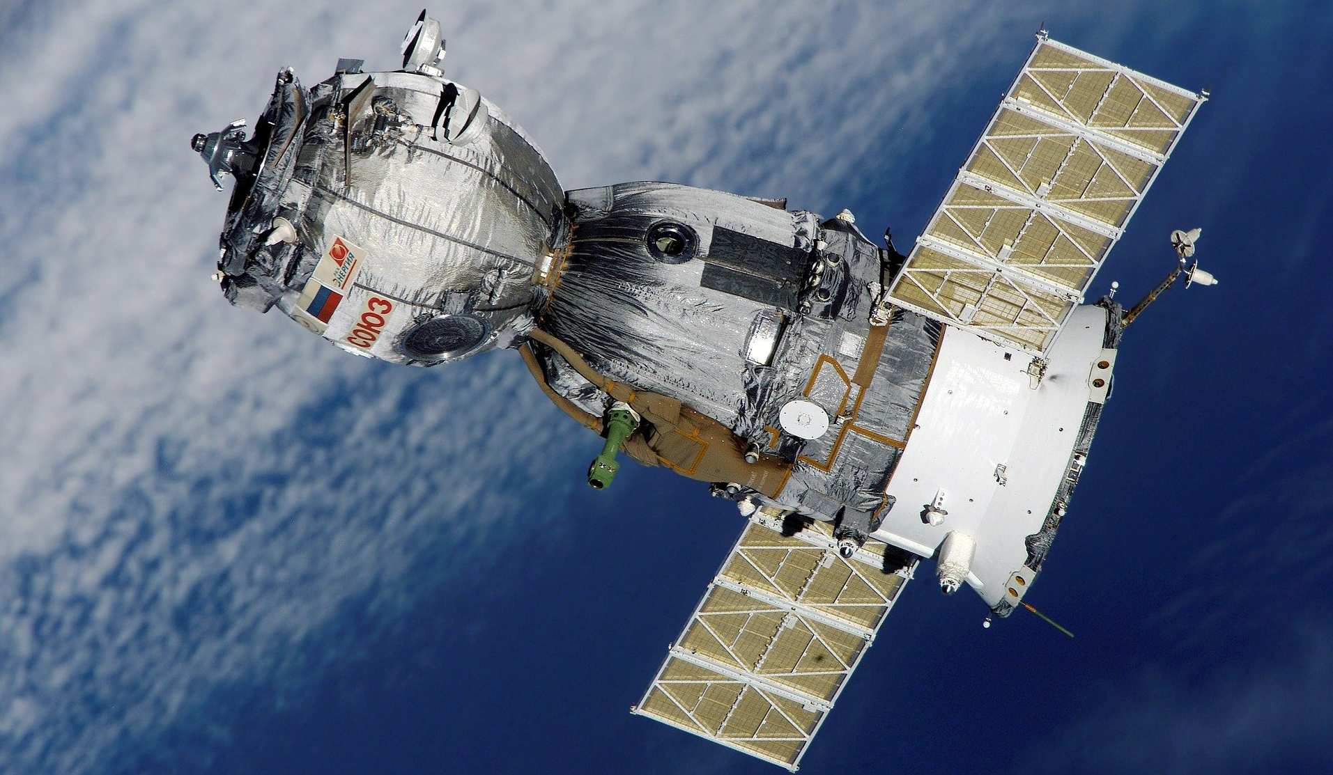
Signal transmission from a GPS (GNSS) medium-earth-orbit (MEO) satellite
The power of GPS signal transmitted from a GPS satellite is about 27 W [see this excellent GPS book]. In decibel unit, the power of the transmitted signal from the satellite is 14.3dBW or 44.3 dBm.
The GPS satellite circulates above the earth at approximately 23000 km. From this very far distance transmission, the main inherent vulnerability of GPS signal is very low power of received signals on a receiver. In addition, GPS and GNSS signals are susceptible to jamming and spoofing attacks.
The power of received satellite signals on the receiver is around -128.5 dBm. That is, the signal power is very low such that the baseband signals containing navigation messages are buried under noise obtained during transmission.
The source of the noise can be from the hardware noise of the satellite transmitter (although this noise should be small as satellites carry high-end instruments), channel transmission (multipath, reflection, path loss, ionospheric delay and others) and the hardware noise at a receiver (depending on the quality of the receiver hardware).
On the satellite side, the signal transmission processing chain for GPS L1 is shown in figure 1 above. From figure 1, the process is as follows. A navigation message is converted into a binary signal with bit values either 0 or 1. This navigation message has a data rate of 50 bit per second (bps).
A Pseudo-random noise (PRN) code that represents a unique satellite number is generated at 1023 chips per 1 ms period. Chip is the same as bit, representing a signal state transition. Commonly the term “chips” refers to bits that do not contain any information. The data rate of the PRN code is then 1.023 million chips per second (Mcps).
A PRN codeis a code with random bits or chips and uniquely represents a unique satellite. This code spreads the spectrum of the navigation message bits. PRN code, in general, has a good autocorrelation and cross-correlation properties. Meaning, when a PRN code is autocorrelated with the same code (prompt correlation), it will have a large correlation value and otherwise for cross-correlation (when the two correlated PRN codes are not aligned together). With this PRN code, the satellite sending the signal can be identified and the signal delay (the time required by the signal to travel from the satellite to the receiver) can be quantified.
Modulo 2 sum operation is applied for the navigation message bit and the PRN code (figure 1 above) so that the spectrum of the message bit becomes wide (spread). The result from this modulo 2 summed signals is then modulated with binary phase-shift keying modulation (BPSK) method. This BPSK modulation will change bit 0 into +1 and bit 1 into -1. The +1 and -1 bits represent positive and negative amplitude of the signals. The actual amplitude value of these positive and negative bits depends on the bit quantisation and the set gain of the transmitting hardware.
In BPSK modulation, the prepared signals are separated into two channels: I (in-phase) and Q (quadrature) channels. The navigation messages, modulated with the PRN code, is in the I channel and only all zero values are in the Q channel. The results of this process are IQ signals.
After the BPSK modulation, the IQ signals are then modulated with the GPS carrier frequency, in this case, 1575.42 MHz (for GPS L1). After the modulation with the carrier signal, the signal is ready for transmission by the satellite.
Figure 2 below shows an example of ideal IQ signals for transmitting (an illustration of signals transmitted by the satellite). Of course, the transmission hardware also has noise. But, the satellite transmission hardware is considered very good and only small noise is added to the ideal IQ signals during transmission.
From figure 2, we can observe that the I channel contains rectangular signals representing (at positive and negative values) the navigation bits. Meanwhile, the Q channel only contains zero values. Figure 2 only shows a snapshot of signals within a short period of time (0.5 s).
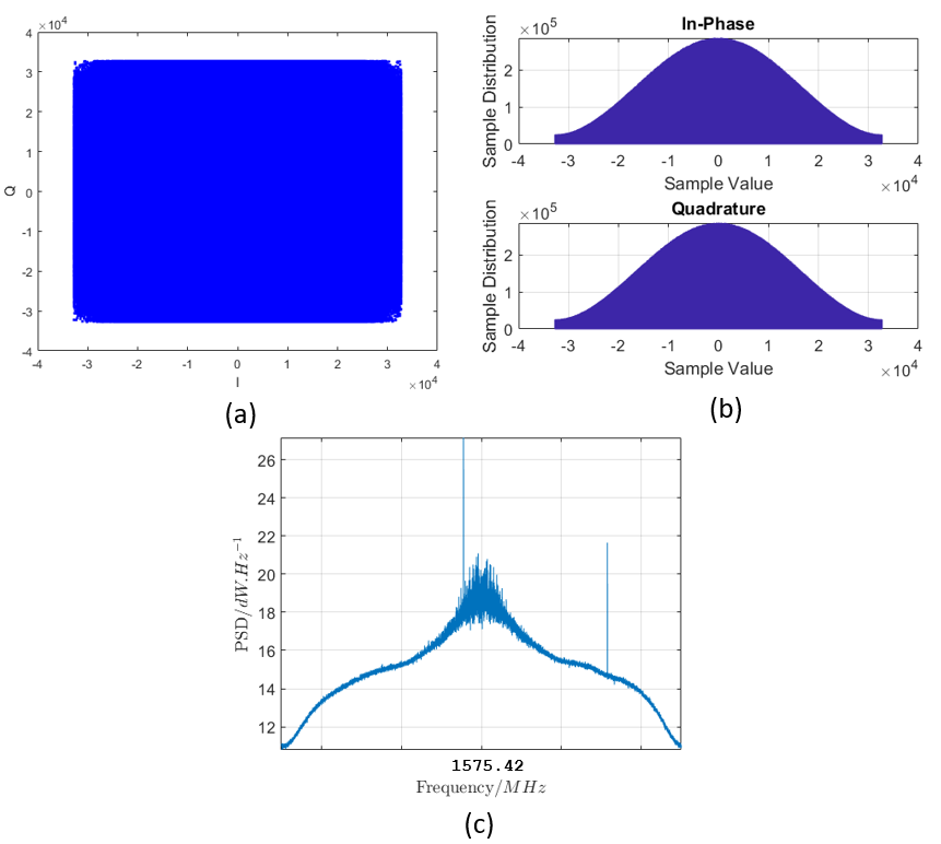
Further analysing the IQ transmitted signals, figure 3 below shows the constellation plot, histogram and the power spectral density (PSD) of the signals. These three steps are the common data inspections applied to analyse all raw IQ signals.
In figure 3a, since the signal is ideal (all zero values in Q channel and only two possible values in I channel), the constellation plot shown only two dots, one in the negative region and the other in the positive region (representing the negative and positive bits, respectively).
In figure 3b, the histogram of the I channel only shows two lines, one in the negative and the other in the positive regions. Meanwhile, the histogram of the Q channel only shows one line at zero.
In figure 3c, the PSD of the IQ signals is shown. As can be observed, there is a main lobe at the centre frequency of 1575.42 MHz representing the base band signal (the navigation message).
The base band signal has 2.046 MHz of bandwidth as the message rate (after adding the PRN code) is at 1.023 Mcps. It is worth to note that we need to carefully quantify signal-to-noise-ratio (SNR) of the signal from a PSD spectrum. Because, the number of bins in the PSD affect the power of the spectrum.
Received signals from the GNSS satellite (Raw I/Q sample)
As being mentioned before, the power of the received signal at the receiver is very low (approximately -128.5 dBm). Hence, the received signal is buried under noises.
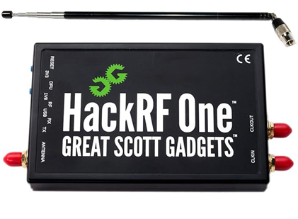
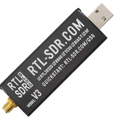
There are many available receiver instruments that we can use to capture GPS (and other GNSS) signals, from high-end instruments such as USRP devices to low-cost instruments that can be acquired by a person for home or personal use, such as RTL-SDRand HACK RF receiver. These RTL-SDRand HACK RF are the most used receiver for home or personal usage.
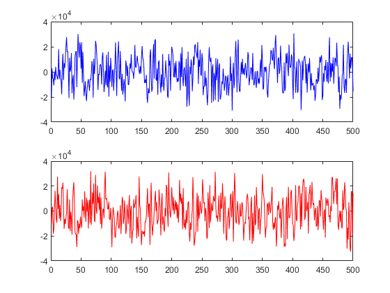
Figure 4 below shows the snapshot (500 samples) of real IQ signals received from a GPS satellite. As can be seen in figure 4 below, the I and Q channel only show noises instead of rectangular signal containing navigation messages (shown in figure 2). The sampling rate at the receiver is 10 MHz, meaning a total of 10 million IQ samples are captured every one second.
From the data inspection of the raw IQ signals received from the satellite shown in figure 5 below, the IQ constellation, histogram and PSD plot of the signals are totally different with the ideal IQ signals.
In figure 5, the IQ constellation shows many dots with a rectangular shape. This shows that all the IQ signals are rotated due to phase shift and their amplitudes vary due to noise. Both the I and Q histograms have a bell-shape curve showing that the signals contain mostly noises (figure 5).
In the next section, how to recover the phase shift (carrier recovery) and how to pull the message bit from the noise so that the bits appear above noise and are ready to be demodulated are explained.
Signal processing chain of the received signal at a GPS (GNSS) receiver
The signal processing chain at the receiver are divided into three steps:
- Signal acquisition
- Signal tracking
- Signal demodulation
These three signal processing chains are mainly to acquire the satellite PRN code to identify what satellite the signals are transmitted from, detect the Doppler shift frequency and the code delay (how long the signal reach the receiver), recover the carrier frequency of the signals (removing the Doppler shift effect), pull the navigation message signals out from the noise (wiping out the PRN code and recover the baseband or message bits) and finally demodulate the navigation message bit.
1. Signal acquisition
This signal acquisition step is to detect the Doppler frequency shift and the code delay form a GPS signal. The detection is by searching a correlation peak across a search space.
The detection of the Doppler frequency and the code delay in this step is only rough estimates and will be refine in the later stage of processing.
The search space is the collection of calculated correlation values calculated from the combination of Doppler frequency shift and code delay. The satellite is considered to be acquired/detected if the highest correlation peak is so pronounced or very high with respect to other correlation values (that is considered as noise). Usually, a threshold value is set so that if a correlation peak is above the set threshold, then a satellite is detected.
When the satellite is detected, the corresponding Doppler frequency and code delay are obtained. These Doppler and code delay estimations are still rough and will be refine in the signal tracking process.
Figure 6 below shows the acquisition search space and the correlation peak with respect to code delay. In figure 6a, from the search space, we can observe clearly that there is a very significant peak compared to other values in the search space bins.
This peak means that the satellite is detected.
A correlation peak is calculated for every 1 ms or more, because 1 ms is the complete period of the PRN code containing 1023 chips. In this case, 10 ms (corresponding to 10 cycle of the PRN code) time period is used to calculate the correlation peak.
The longer the time used to correlate the PRN code, the higher the noise suppression, but the longer the time required to detect the satellite. So, this time period to calculate the correlation peak is a trade-off decision depending on applications.
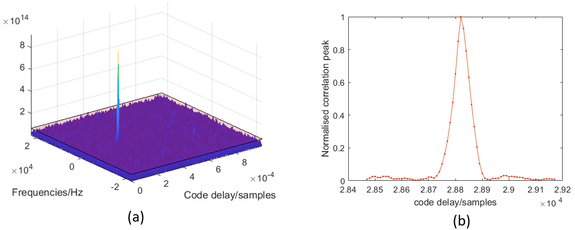
The calculation of the correlation peak is by integrating (correlating) a local copy of the PRN code at the receiver with the received signal to find what delay the local PRN aligned with the PRN code from the received signals.
From figure 6b above, we can see that when the local copy of the PRN code is aligned to (have the same delay with) the PRN code in the received signals, the correlation value becomes significantly high. Any slight misalignments between the local PRN code and the PRN code in the signals will significantly reduce the correlation value.
In a perfect condition, the correlation peak has a perfect triangle shape. The more noise contained in received signals, the more deviation from a perfect triangle shape the correlation peak will be.
2. Signal tracking
If the satellite is detected and the Doppler frequency and code delay can be roughly estimated, the signals will be processed further in the signal tracking stage.
The main goals of this signal tracking are to track (fine estimate) the Doppler and the code delay and to prompt correlate the local copy PRN code with the signals to pull out the message signals from the noise.
The Doppler and code delay are change in time. Because, the satellite, and very often, the receiver are in motion. That is why, the Doppler frequency and the code delay should be track in time.
The tracking process is commonly every 1 ms (one period of the PRN code). But, it can be more than 1 ms.
The estimated Doppler frequency is used to recover the carrier phase and the prompt code delay is used to wipe out the PRN code from the message signals (de-spreading the signal).
Figure 7 above shows the tracking process of the signals after the satellite is detected. In figure 7a, the Doppler and code delay can be detected after less one second.
These tracked Doppler frequency and code delay are used to recover the carrier phase and then to prompt correlate the local PRN code with the signals (wiping out the PRN code) to pull out the message signals.
The carrier tracking loop uses Costas loop in the implementation. The idea of Costas loop is to put all the signal power on the I channel and remove all the power from the Q channel.
In figure 7b above, the tracked I channel shows rectangular shape signals representing the message signals and the Q channel show values around zero because there are no messages in the Q channel and only noise signal left in the Q channel.
3. Signal demodulation
Finally, after the signal tracking, the message bit can be demodulated. The demodulation is applied to the prompt correlated (tracked) I signals shown in figure 7b above (in red).
From the tracked I signals (in figure 7b in red), the demodulation process is carried out by integrating the bit values for every 20 ms. If the value of the integration is > 0 (positive), hence it is recognised as bit 0 navigation message bit and other wise (remember due to BPSK modulation 0 bit becomes +1 or positive and 0 bit becomes -1 or negative).
The 20 ms integration time is because the rate of the navigation message bits is 50 bps, meaning every single navigation bit has 20 ms period.
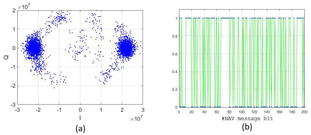
Figure 8 below shows the IQ constellation after the tracking and the demodulated message bit. In figure 8, we can see that the carrier and the message signal (in I signals) can be recovered as these signals are aligned at Q = 0 and are clustered into two groups: positive and negative (along the I axis).
Figure 8b shows the demodulated 0 and 1 navigation bits. From these 0 and 1 bits, the navigation message can be recovered.
To better see the evolution of the IQ signals from the transmission at the satellite, received at the receiver until the signal tracking process, figure 9 below compares the IQ constellation plot for transmitted, received and tracked (ready for demodulation) signals.
As can be seen from figure 9, the tracked IQ constellation (right) can be recovered from the noisy IQ signals (middle) received at the receiver. The tracked IQ constellations resemble the two constellation groups as shown in the ideal IQ constellation (left).
The points outside the two clusters in the tracked IQ constellation (figure 9 right) are due to the transient period of the tracking process before locking the carrier (Doppler) and code delay (shown in figure 7a).
Signal comparisons at different transmission modes
It is good if we can see signals evolution if the transmission is sent via a cable or close-range wireless transmission, instead of being sent from a satellite. By this comparison, we can have a picture on how low the power and how noisy the received signals transmitted from a satellite.
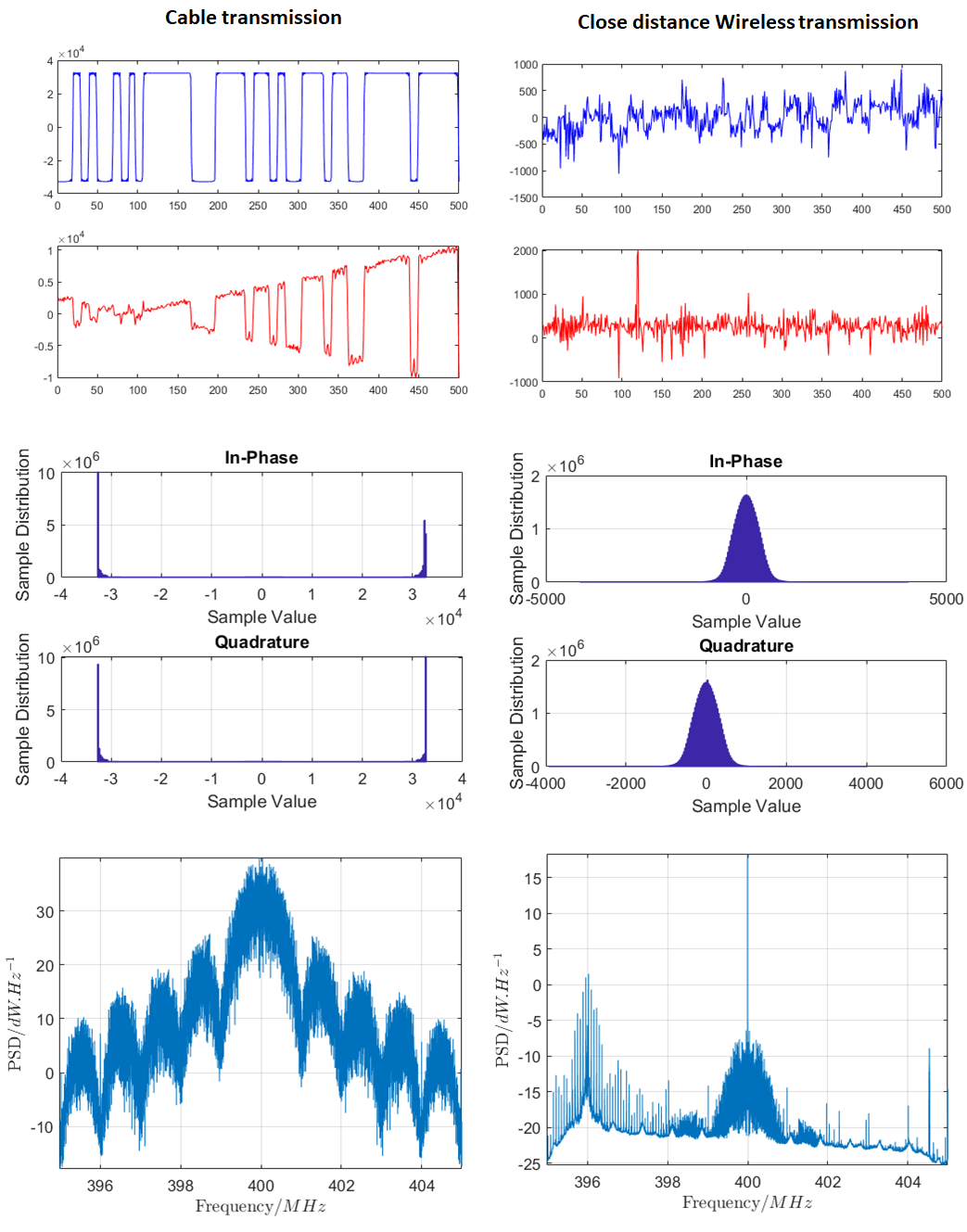
Figure 10 below shows the received GPS signals from the cable and wireless transmission performed in a laboratory test. The carrier frequency for the test transmission is 400 MHz.
In figure 10a, a clear rectangular shape on the I channel can be observed. Meaning, the message signals are not buried under noise.
Because, with cable, the transmission is via a physical channel that has very low channel noise. In addition, the histogram shows the two lines representing the message bits.
In figure 10a, some signals can be observed on the Q channel as some power are distributed to Q channel during transmission process. The signal amplitude on Q channel is much lower than the amplitude on the I channel.
Figure 10b shows the received IQ signals from the wireless transmission. The distance between the transmitter and receiver is about < 20 m. As can be seen in figure 10b, because the wireless transmission has more noise (due to for example, path loss, multipath and reflection) compared to the cable transmission, the I signals deviate from a rectangular shape. However, we still can observe somehow the message signals in the I channel.
From the histogram in figure 10b, the histogram starts to have a bell-shape showing that the noise signals are more dominant than the message signals.
Both the PSDs show the main lobe of the base band signal at the centre frequency of the carrier (figure 10). The main lobe has 2.046 MHz width representing the baseband signals. The total signal bandwidth is 10 Mhz following the sampling rate at 10 Mhz.
The comparison of signal acquisition of the received signals between the cable and wireless transmission is shown in figure 11 below.
In figure 11, we can see that the acquisition search space from the wireless transmission has higher noise than the cable transmission. However, in both conditions, the satellite signals can still be detected.
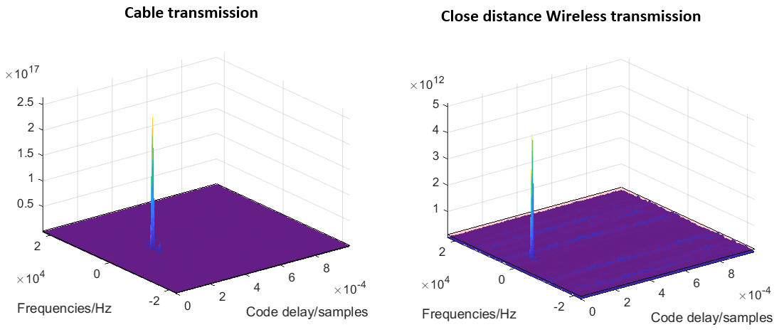
Figure 12 below, the comparison of the signal tracking from both the cable and wireless transmission is shown. As can be seen in figure 12 right, the tracking of the signals received from the wireless transmission is noisier compared to the signals received from the cable transmission. The tracked Q channel can clearly show the noise content in the received signal from the wireless transmission.
From the tracked IQ constellation in figure 12, we can observe that the cluster of the points on the wireless transmitted signals have a larger size than the cable transmitted signal due to more noise content in the signal.
The wireless transmission has more channel impairments that add noise to the signals.
Comparison of different integration time for signal acquisition
In signal acquisition stage, a long integration time (the time period to calculate the correlation of the local PRN with the PRN code of received signals) can be applied to suppress noises on received signals. However, there is a trade-off between noise suppression and computation efficiency when determining the integration time.
The longer the integration time, the higher the noise suppression capability, but, the higher and longer the computation cost and time.
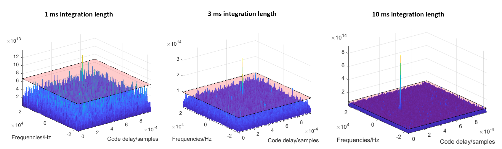
Figure 13 below shows the comparison of the acquisition search spaces obtained with 1 ms, 3 ms and 10 ms integration time. In figure 13, with 10 ms integration time, the noise can be significantly suppressed compared to 1 ms integration time.
Considering the trade-off, the integration time of 3 ms can be selected in this case. Because, with 3 ms integration time, the correlation peak can be clearly seen and we can save some computation power.
Conclusion
This post focuses on explaining the evolution of GPS signals from transmission at a satellite all the way to receiving, acquiring, tracking and to demodulating the navigation message signals.
The explanations show various signal plots so that readers can understand what are happening on the GPS signals in each step during the signal processing chain.
In addition, the comparisons among signals received from a satellite, a cable transmission and a close-distance wireless transmission are presented so that reader can clearly see how low the power and how noisy are received GPS signals.
Finally, the beauty of signal processing chains at a GPS receiver can recover and pull out useful navigation message signals buried under noise due to channel and hardware (especially the receiver) impairments during transmission.
- We recommend the book of Prof. Eisenhardt about “Simple rules: How to thrive in a complex world”.
- In addition, We also recommend books “Deep Work: Rules for Focused Success in a Distracted World” about how to do work that give big results by Cal Newport.