Mathematical geometrical fitting: Data filtering of measurement points

Data filtering is a process to reduce noises or suppress certain components or information contained in measurement data by using a specific kernel (filter).

Noises are undesired data contained in measurement data and are caused by uncontrolled conditions during measurement processes, for example, temperature variation and vibration noise.

The formal definition of a filtering process in dimensional and geometrical measurement is the process to differentiate various types of effects that occur in various types of scales of length unit [1].

In general, filtering process is divided into two classes:

• Filtering based on convolution (linear filtering)
• Filtering based on morphological operation (non-linear filtering)

In the case of tactile and optical coordinate measuring machine (CMM) and stylus instrument, many measured points obtained by these instruments contain noises that manifested into points that do not represent the actual profile of a measured surface.

For example, very often, the noises can be found in term of a sudden jump on the height of the measured points. Hence, a filtering process is used to remove this sudden-jump point so that the calculated measurement result from the measured points can be accurate.

In this post, the two types of filtering will be discussed and examples are given.

READ MORE: Mathematical geometrical fitting: Concept and fitting methods

Filtering based on convolution (linear filtering)

Filtering based on convolution is a linear filtering process that uses a certain kernel with a specific “window” size. Convolutional based filtering is a linear mathematical operation and is the most common type of filtering processes.

The kernel of a convolutional filter is applied to all measured points for a measurement process. The kernel is convoluted to these measured points by the following formula:

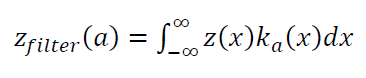
Where $Z_{filter} (a)$ is the filtered $z(x)$ values, $z(x)$ is the $z$ value (height) of a position $x$ and $k_{a}(x)$ is a kernel with certain window size (width) that is centred at $a$.

Filtering process based on convolutional operation is also called as “mean” filter. Because, in principle, this type of filter averages a value form several measured values.

Since a convolutional filter will pass data with low frequency component characteristics, such as waviness and form data, this convolutional filtering is also called low-pass filter (passing data with low frequency components and block data with high frequency components).

A simple example of filtering process based on convolution is as follows.

Let we measured the profile of a surface and get the height of the profile as $[1,2,1,2,1,2,1,2]$ that is eight measurement points.

If a convolutional filter is applied to these eight points with kernel size of three (covering three points that are the interested point, left point and right point) with equal weight, then the filtered data will be $[4/3, 5/3, 4/3, 5/3, 4/3,5/3]$.

The filtered data becomes only six points because the point at the two edges cannot be calculated due to the kernel requirements. This situation is called “edge effect”.

The above filtering process example is equal with performing a convolution process (as in the equation above) on data $[1,2,1,2,1,2,1,2]$ with a kernel $[1/3,1/3,1/3]$.

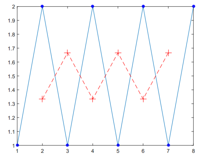
Figure 1 above shows the plot of the initial data and the filtered data of the simple example. In figure 1, the initial eight data are shown with symbol “.”. Meanwhile, the filtered data is shown with symbol “+”.

It can be seen in figure 1 that the filtering results are the average of the three initial data and have lower value than the initial data before filtering. These smaller values than before filtering are due to the averaging process of the convolutional filter.

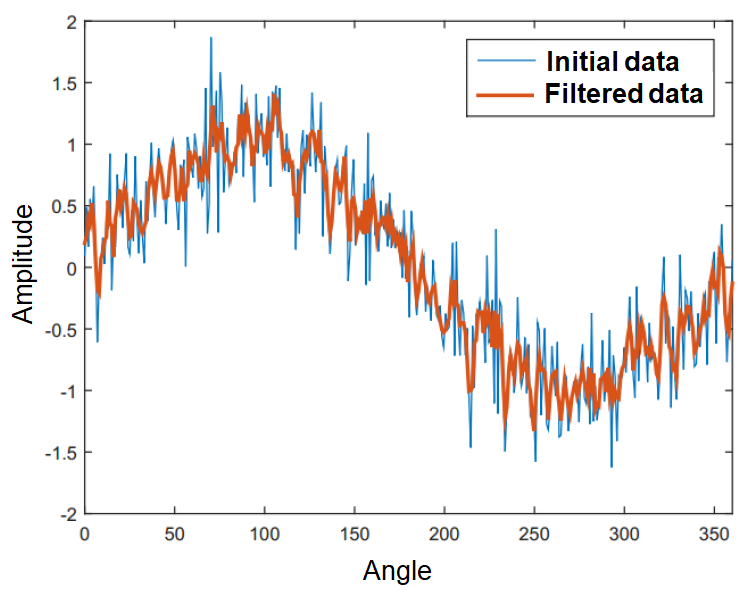
Another example of convolutional filtering is shown in figure 2 above. In figure 2, a sinusoidal curve containing high noise if filtered by convoluting the data with kernel $[1/3,1/3,1/3]$. As can be seen from figure 2, the filtered data lies in between the non-filtered data due to the averaging effect.

Figure 3 below shows an example of convolutional filtering applied to 2D data (image data). Since the data is 2D, the filter kernel is also 2D and is defined as:

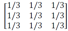
Hence, this 2D kernel is applied to the 2D data (image) and calculate the weighted-averaged value from the original data that are covered by the kernel size.

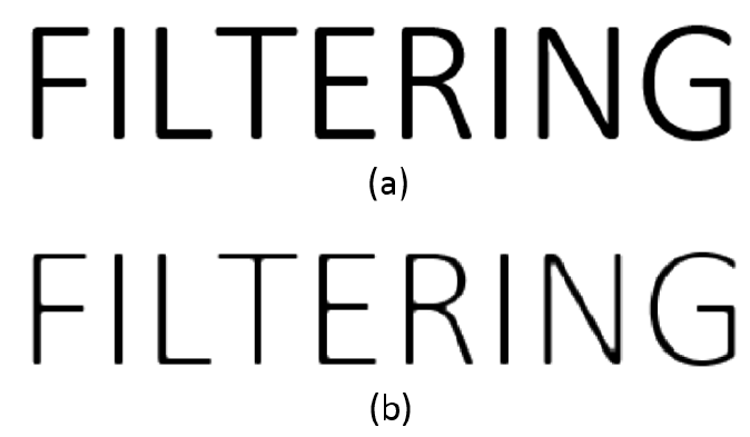
In figure 3 below, an image of a word “FILTERING” is used as the example. The kernel is convoluted with this image. The results of the filtering process are a blurred version of “FILTERING” image.

The “blurring” effect is due to the high frequency component of the images is supressed by the convolution filter. High frequency components in an image are “sharp” features, such as sharp edges.

These sharp features will be supressed and then become “blur”. That is, only low-frequency components in the data are passed out from the filter.

READ MORE: Mathematical geometrical fitting: Linear geometry least-squared fitting (with tutorial)

Filtering based on morphological operation (non-linear filtering)

Morphological filter is a type of non-linear filter. This type of filter also has a kernel. However, the kernel is not an averaging operation.

There are two main types of morphological filter that are:

• Dilation
• erosion

Dilation is a morphological filter of which when its kernel with a certain length and width passes a point or data, hence all points in the area covered by the kernel is a new set of data.

Otherwise, erosion is a morphological filter of which when its kernel with a certain length and width passes a point or data, hence all points in the area covered by the kernel is out of the point set.

For simplicity and intuition, dilation filter is like a paint brush that colour the area along a line trajectory and erosion filter is like an eraser.

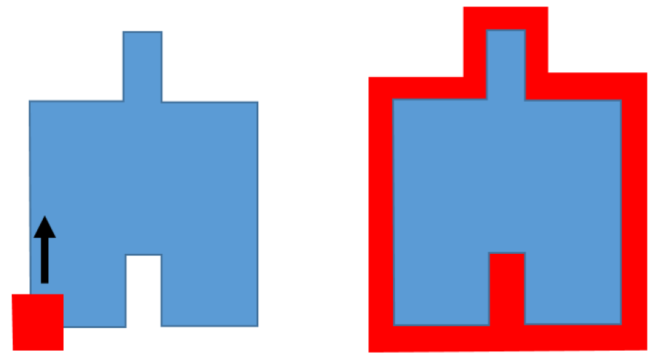
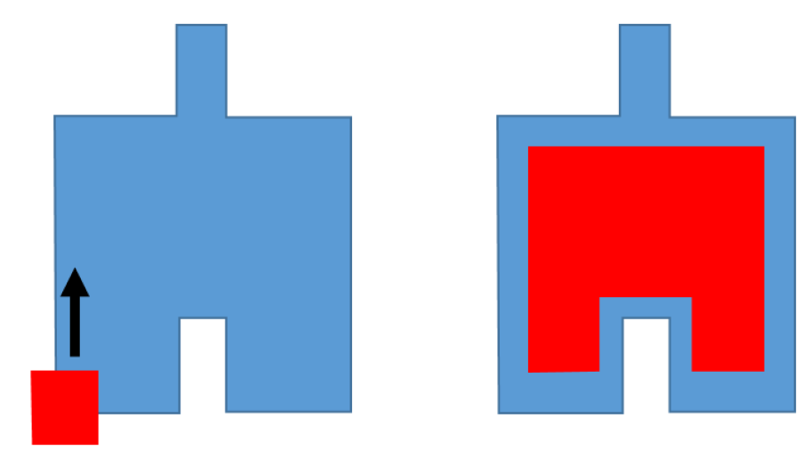
Figure 4 above shows an example of dilation operation. In figure 4, it can be observed that the area passed by the dilation kernel becomes active. Hence, the filtered shape has a bigger size before the dilation filtering operation. Note that from this dilation process, the small feature of the shape can be closed!

Figure 5 above shows an example of erosion operation. In figure 5, the area passed by the erosion filter becomes inactive. In other words, the filtered shape becomes smaller than before the erosion process.

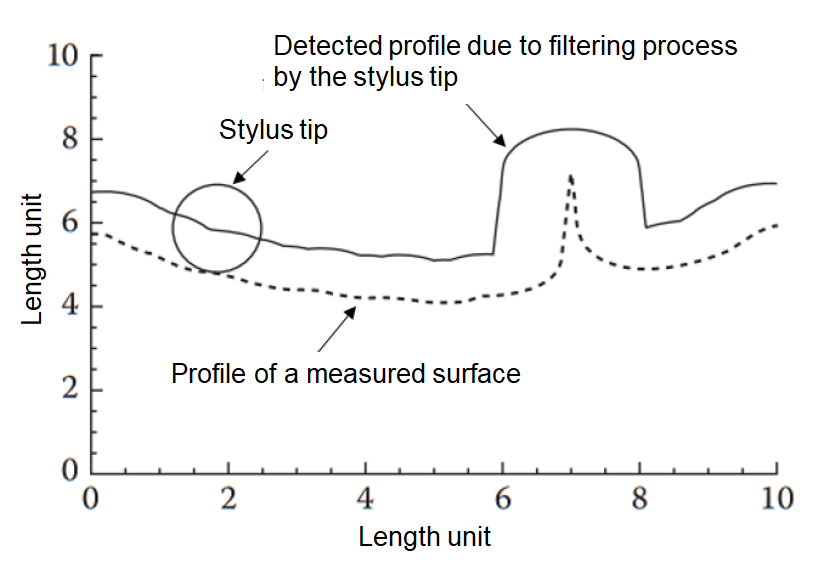
In the case for dimensional and geometrical as well as surface texture measurements, morphological filter operation is very relevant to simulate the trajectory of a small sphere rolled over a measured surface (that is simulating the tip of a tactile or contact instrument touching the measured surface).

All measured points from a tactile or contact instrument are actually the location of the centre of the tip of the instrument passing through a measured surface. That is, all measured points from the instruments are actually have been morphologically filtered (physical morphological filter).

Figure 6 below shows the physical morphological filtering process performed by a stylus tip on the profile of a measured surface. From figure 6, it is very clear that the measured profile is not the same with the real surface due to the morphological filtering process of the stylus tip.

Finally, besides the most common types of filtering, convolutional and morphological filtering, discussed in this post, there are other types of filtering, such as median filtering, high-pass filtering, band-pass filtering and other types of filtering.

READ MORE: Mathematical geometrical fitting: Non-linear geometry least-squared fitting (with tutorial)

Conclusion

In this post, the concept and examples of filtering processes are explained. Two very common filtering process that have been discussed are convolutional filtering and morphological filtering.

These two filtering processes are very relevant for dimensional, geometrical and surface texture measurements.

Convolutional filtering is very use full to supress high frequency noise commonly found in measurement data.

Especially for contact or tactile measuring instrument, morphological filter is relevant to model and understand the effect of the size of the tip of the instrument when measuring the profile of a surface.

References

[1] Hocken, R.J. and Pereira, P.H. eds., 2016. Coordinate measuring machines and systems. CRC press.

You may find some interesting items by shopping here.