Measurement uncertainty estimation: Spreadsheets method

This post will discuss Spreadsheets method to estimate measurement uncertainties. This method is the most well-known and used method to estimate measurement uncertainties.

Spreadsheets method can be used for any types of measurement with or without the availability of measurement mathematical models.

(Readers may read the previous posts regarding measurement uncertainty estimations with GUM method and Monte-Carlo simulation method)

Let us go in detail!

Spreadsheets method

The spreadsheets method is, perhaps, the most well-known and used method to estimate the measurement uncertainty of any types of measurement results.

Spreadsheets method use a table to list all the factors considered relevant to a measurement result and uncertainty and manually sum-of-square them together to estimate the total uncertainty.

This spreadsheets method is one of the alternative of the GUM method to estimate measurement uncertainties. Another GUM alternative is the Monte-Carlo method.

Spreadsheets method is mostly used when the exact mathematical model or the differentiable mathematical model of a measurement is not available.

Also, Spreadsheets method considers all relevant factors affecting measurement results and uncertainties. Hence, when the mathematical model of a measurement is not available, expertise or experiences of the measurement are required to determine the relevant factors.

The elements of spreadsheets method to estimate measurement uncertainty

The main elements of the spreadsheets table to estimate uncertainty are as follow:

• 1. The uncertainty sources or factors, for example repeatability, reproducibility, temperature variation, pressure variation and humidity variations
• 2. Interval value ($\pm$) or $u(X_{i})$. This value is the estimated uncertainty for each factor $X_{i}$ that contributes to a total uncertainty
• 3. Value conversion and sensitivity coefficient $C_{i}$

The conversion process is a process to convert the unit of an uncertainty contributor $X_{i}$ if this contributor has a unit that differs from the unit of measurement $Y$. For example, the measurement results is a length in mm and the contributor $X_{i}$ is temperature in Kelvin.

For the conversion process, the direct calculation method, that is a partial derivation of $Y$ with respect to $X_{i}$ is calculated. A conversion using this direct calculation or partial derivative is calculated as follow:

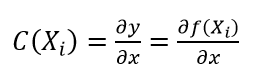
We can use the equation above when we have the model of a measurement. Meanwhile, when we do not have the measurement model, we can estimate the derivation as follow:

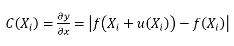
When the unit of $u_{Xi}$ is already the same with the unit of $y=f(X_{i})$ (that is the measurement unit), this convention process is not needed.

Otherwise, we need to estimate $u_{Xi}$ as $u_{Xi}=C(X_{i}) . u(X_{i})$.

When a measurement model is not known, we can use the numerical derivation above.

The sensitivity coefficient is a coefficient that describes how large a uncertainty contributor $X_{i}$ affects the measurement results $Y$. This sensitivity coefficient is obtained from the constant of the variables from the partial derivation of $Y=f(X_{i})$ with respect to $X_{i}$ (as just mentioned above).

For example, we have a measurement model of depth measurement as:

Where $D$ is measured depth with unit $m$, $v$ is measured velocity with unit $m/s$ and $t$ is measured sound travel time with unit $s$. From the model above, the uncertainty factors $X_{i}$ for $D$ is $v$ and $t$. Since $v$ and $t$ have different unit with respect to $D$, hence the $v$ and $t$ should be applied a conversion process.

The conversion process for both $v$ ad $t$ are:

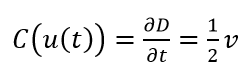
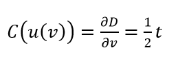
Hence, we multiply the varied value of $v$ and $t$ to the corresponding equation above $ C(u(t))$ and $ C(u(v))$ to convert the unit to $m$. $u_{t}=C(u(t)).u(t)$ and $u_{v}=C(u(v)).u(v)$ both have unit in $m$ and the coefficient sensitivity for both of them are $1/2$.

For measurement that the model is unknown, the coefficient sensitivity is commonly assumed to be 1 and the derivation is using the numerical method mentioned above $f(X_{i}+u(X_{i}))- f(X_{i})$.

• 4. The probability distribution from the uncertainty factor $X_{i}$ at point 1.
• 5. Divisor $d_{i}$

This divisor depend on statistical distributions assumed for the uncertainty contributor.

• 6. Standard uncertainty

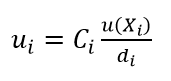
Table 1 shows a spreadsheets table that contains the elements required to estimate uncertainty using this method. Table 2 shows the list of divisor $d_{i}$ (element #5 above) for several statistical distributions commonly used practically.

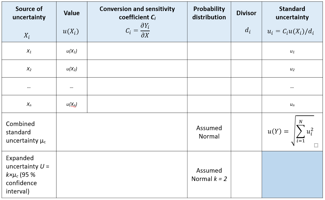
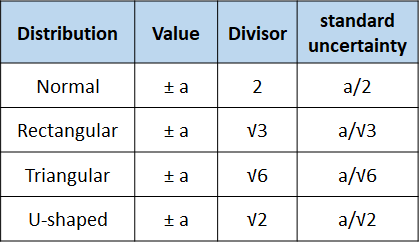
For type A uncertainty, normal distribution is used. Meanwhile, for type B uncertainty, common used distributions are rectangular distribution (usually for uncertainty factors from calibration values or from dimensional tolerance), triangular and U-shape.

For the sensitivity coefficient $C_{i}$, commonly the value is assumed to be 1 for type B uncertainty and for a case when we do not have the mathematical model of a measurement with respect to an uncertainty factor of interest. When the model is known, $C_{i}$ will be calculated from the derivation between $Y$ and $X_{i}$.

To understand clearly the use of spreadsheets method to estimate uncertainty, next sections will present some examples that are common in industry and measurement practices.

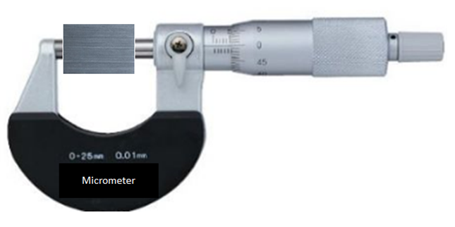
Example 1: the measurement uncertainty of 50 mm gauge block measurement with a micrometer

In this example, the measurement uncertainty of the calibration of a micrometre with a 50 mm gauge block is presented. The calibration is performed by measuring a 50 mm calibrated gauge block. Figure 1 shows the micrometre calibration process with the 50 mm gauge block.

The mathematical model of this measurement is formulated as:

Where is $L$ the measured gauge block length, $X_{read}$ is the scale resolution of the gauge block, $\alpha$ is the thermal expansion coefficient of the gauge block, $T$ is the temperature when a measurement is performed.

The first step to estimate the measurement uncertainty is to list all relevant uncertainty contributors that affect the gauge block measurement with the micrometre.

These relevant factors can be obtained from the measurement model (in this case is available), calibration certificates and/or from expert judgments.

For this measurement, the uncertainty contributing factors are:

• The uncertainty of the measured gauge block (from the gauge block calibration certificate)
• The resolution of the micrometre
• The standard deviation of mean from repeated measurements of the gauge block with the micrometre
• The variation of measurement temperature (related to the thermal expansion of the measured gauge block)
• The error of the thermal expansion coefficient of the measured gauge block

Hence, based on the list of the uncertainty contributing factors, the uncertainty budget and estimation of this measurement are formulated and presented in table 3.

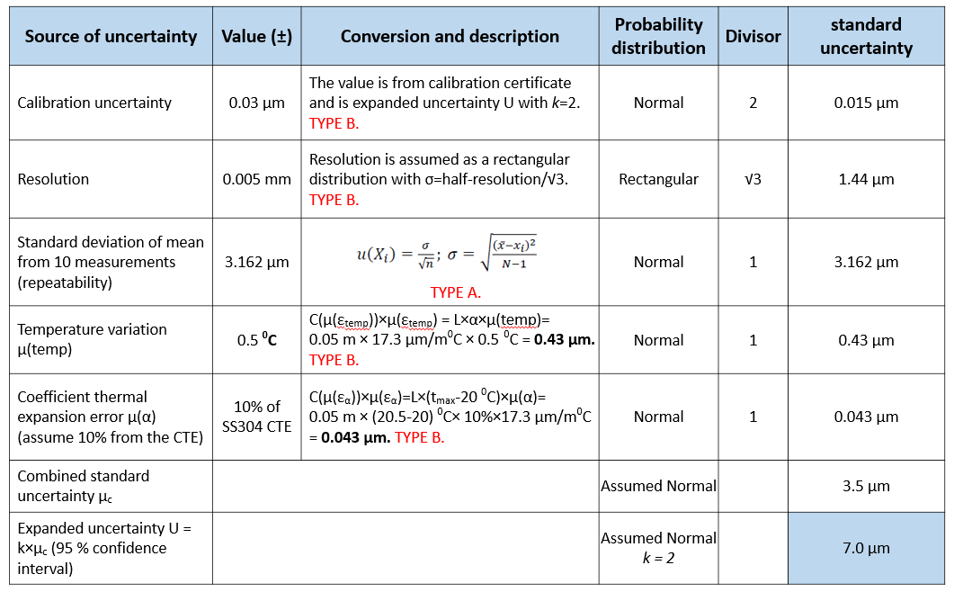
The detailed explanations of the uncertainty budget and estimation in table 3 are as follow:

• The uncertainty from gauge block calibration

Any calibrated (reference) artefacts should have their own calibration certificate issued by approved calibration laboratories. In a calibration certificate, the extended uncertainty of the calibration will be stated. In general, the uncertainty is assumed to be normally distributed (Gaussian distribution) so that to get the $u_{i}$ we just need to divide the extended uncertainty by 2 (see table 2 above).

• The uncertainty from the scale resolution of the micrometre

The uncertainty of the scale resolution is always one of the uncertainty factors of a length measurement system. Due to resolution limitation, a measurement results that lies in between two scales cannot be determined. The uncertainty due to this resolution limitation in general is assumed to follow rectangular distribution so that the $u_{i}$ is calculated as half-of-the-resolution divided by $\sqrt{3}$ (see table 2 above).

• The uncertainty from the repeated measurements (repeatability): standard deviation of the mean

From the uncertainty source from measurement repeatability, the standard deviation from the mean is used to estimate the uncertainty contribution of the repeatability. It is important to note that standard deviation of the mean is different with the standard deviation. The uncertainty source from the measurement repeatability also includes other uncertainty contributors that are not included in table 3 above, for example, an uncertainty contribution from the mistake or the inaccuracy of operator readings.

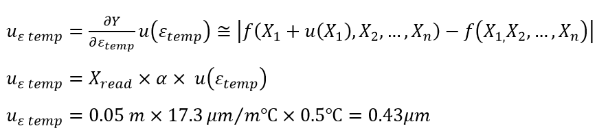
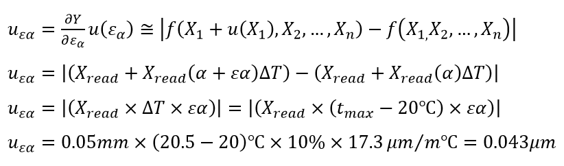
• The uncertainty from temperature variation when measuring

For the uncertainty from temperature variation, the uncertainty has a different unit, that is degree $C$ with measured length, that is $\mu m$. Hence, the unit conversion process needs to be applied. To convert the unit of the uncertainty from temperature variation (and also from the coefficient of thermal expansion) to the unit of length in $\mu m$, the partial derivation or direct calculation method should be applied. The method can be applied for single or multiple variable models, as follow:

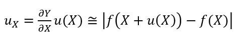
Single variable model:

A measurement model (function) $Y=f(X)$, where $X$ has a unit that differs to the unit of $Y$. Hence, to convert the unit of the uncertainty of $X=u(X)$, the $u_{X}$ (after unit conversion) is calculated as:

Multivariable model:

A measurement model (function) $Y=f(X_{1}, X_{2},…, X_{n})$, where $X_{i}$ has a unit that differs to the unit of $Y$. Hence, to convert the unit of the uncertainty of $u(X_{i})$, the $u_{Xi}$ (after unit conversion) is calculated as:

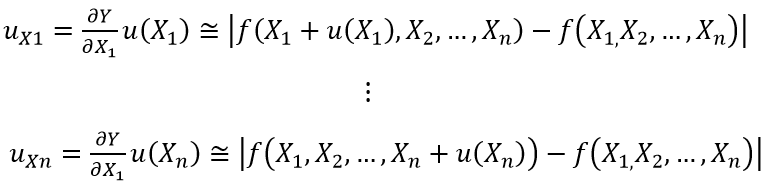
Or, In general:

Hence, the conversion of temperature variation with respect to gauge block length of 50 mm is:

• The uncertainty from the thermal expansion coefficient of the gauge block

Similarly, the unit conversion for the uncertainty contributors of the thermal expansion coefficient variation $\epsilon \alpha$ with respect to the 50 mm gauge block length is calculated as:

Finally, the measurement results of the 50 mm gauge block measurement with the micrometre can be completely reported as:

• The length of the gauge block = $Y=(50 \pm 0.007) mm$
• The interval of 0.007 mm is the expanded uncertainty with $k=2$ that covers 95% confidence interval (assumed to be normally distributed)
• The length 50 mm is the average from 10 repeated measurements. The uncertainty value is estimated by using Spreadsheets method. The measurement was performed in a controlled laboratory at $(25 \pm 0.5)$ degree C by an experienced operator

Example 2: the measurement uncertainty of a density measurement of a solid sphere with volume V and mass m

In this example, the measurement of the density $\rho$ of a sphere is presented. The measurement model of this density measurement is:

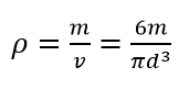
From the above measurement model, it can be observed that the contributors of the density measurement are the mass $m$ and diameter $d$ of the sphere.

Let us say that the average of the measured $\rho$ is calculated from the averaged measurements of $m$ and the sphere diameter $d$ from, let say, five measurements, is as follow:

• The averaged value of $d$ is 2.475 cm
• The averaged value of $m$ is 19.7 g
• From the given $m$ and $d$, the density $\rho$ is estimated as $\rho = 2.49 g/cm^{3}$

The budget and estimation of the measured density uncertainty by using Spreadsheets method is shown in table 4.

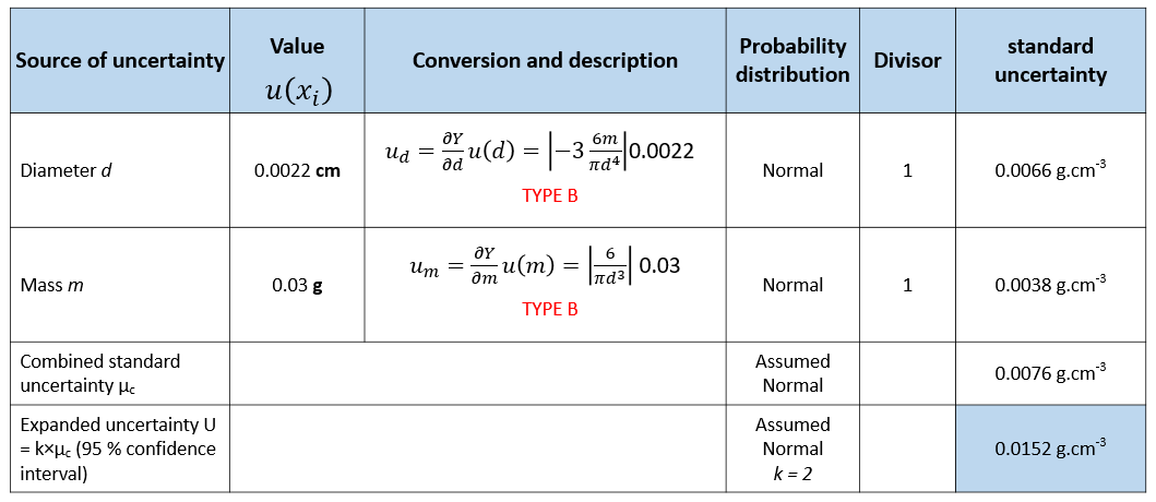
In table 4 above, there are two main uncertainty contributors as previously mentioned: the mass $m$ and the diameter $d$.

From the uncertainty contributor $d$, it can be observed that $d$ has an order 3 in the density measurement model above. Hence, the partial derivative $\rho$ with respect to $d$ has a coefficient of 3.

Note that in table 4, the uncertainty for repeatability is not presented and is assumed to be very small (negligible) with respect to other uncertainty contributors.

Finally, the complete presentation of the results of the density $\rho$ measurements are:

• The density of the sphere $= (2.49 \pm 0.0152) g.cm^{3}$
• The interval is $0.0152 g.cm^{3}$ is the expanded uncertainty with a coverage factor $k = 2$ (95 % confidence interval, assumed Normal distribution)
• The density of $2.49 g.cm^{3}$ is the mean from 5 times repeated measurements. The uncertainty was estimated by spread sheet method.

Conclusion

In this post, the most well-known and used method to estimate uncertainty has been discussed.

The method is spreadsheets method that considers all important factors of a measurement and arrange them in term of a table with a certain structures.

This method is most preferable because at least for two reasons:

• This method does not require the analytical and derivable mathematical model of a measurement. Because, most of the time, the model is very complex and is not available or not known
• This method does not need a computer or programming to estimate measurement uncertainties

From this post, readers can applied this method to estimate measurement uncertainty for any types of measurement in any fields.

We sell all the source files, EXE file, include and LIB files as well as documentation of ellipse fitting by using C/C++, Qt framework, Eigen and OpenCV libraries in this link.

We sell tutorials (containing PDF files, MATLAB scripts and CAD files) about 3D tolerance stack-up analysis based on statistical method (Monte-Carlo/MC Simulation).