Ten types of dimensional and geometrical measurement error

In any dimensional and geometrical measurements, different types of measurement error decrease the accuracy of the measurements. These types of measurement error can be classified into two general categories:

• Measurement error related to measurement procedures
• Measurement error related to structural elements of measuring instruments

Examples of error related to measurement procedures are Abbe error, Sine and cosine error, datum error, zeroing error, misalignment error, error due to surface roughness and non-technical error.

Meanwhile, examples of error related to structural elements of instruments are geometrical error, non-kinematic design error, dynamic error, control error, structural loop error, component’s material expansion error and environment related error (such as errors due to dust and dirt).

These types or measurement error are explained as follow:

1. Abbe error

Abbe error is the most fundamental error in dimensional and geometrical measurements. The name “Abbe” is due to the person, Ernst Abbe, who observed the error for the first time. Ernst Abbe is the first engineer working at ZEISS.

Abbe error is caused due to the measurement axis and motion axis of a measuring instrument do not coincident each other. These two non-coincident axes cause any small angular errors of the measuring arm of the instrument will be amplified and translated into Abbe error (figure 1). The magnitude of the amplified Abbe error depends on how large the Abbe offset of the instrument has (see figure 1).

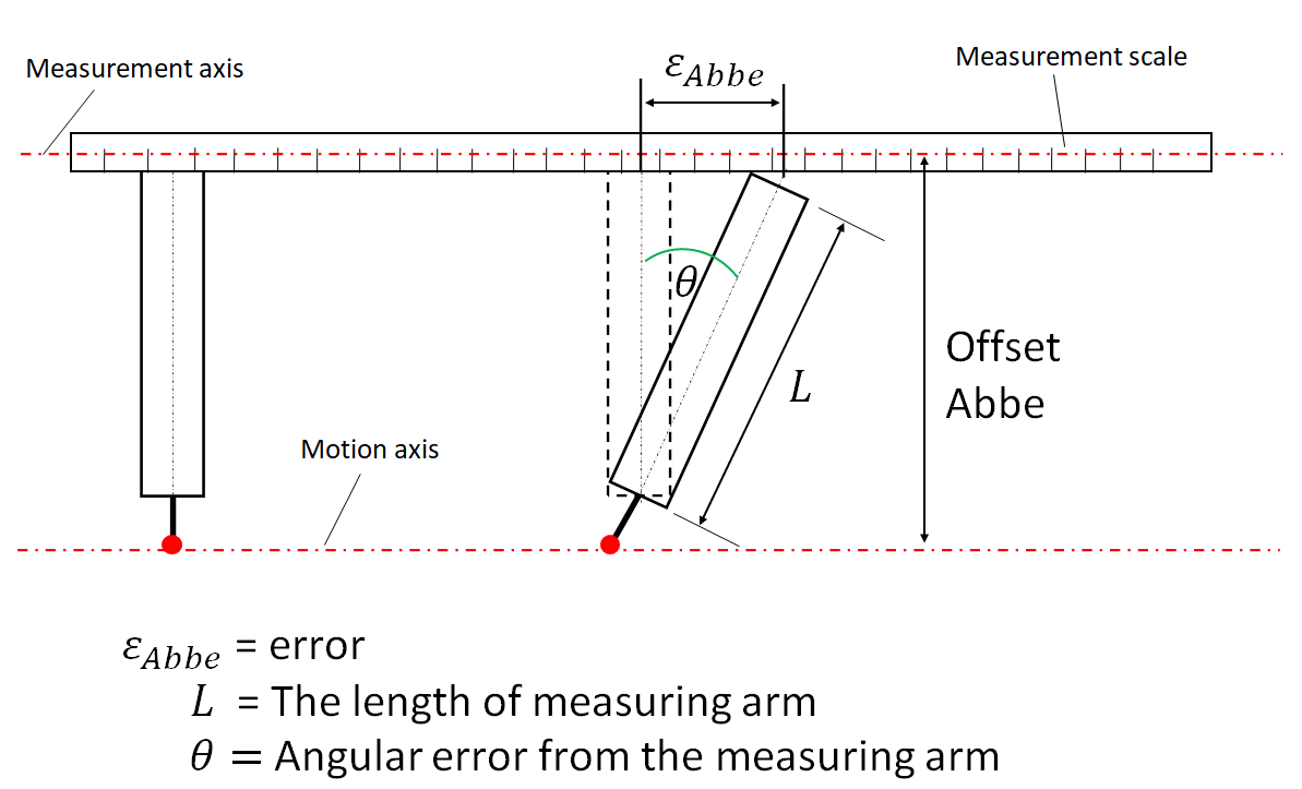
Abbe offset is the distance between the non-coincident measuring axis and motion axis of an instrument. The motion axis is the axis where the instrument moves during operation and the measurement axis is the axis where the measurement scale, from where a measurement reading is taken, is placed.

Figure 1 shows the illustration of Abbe offset, Abbe error, measurement axis, motion axis and angular error of an instrument. In figure 1, Abbe error is calculated as:

$\epsilon _{Abbe}=\epsilon _{offset}\times \tan (\theta)$

where $\epsilon _{Abbe}$ is Abbe offset and $\theta$ is angular error.

In figure 1, an instrument having a measurement arm length of $L$ and a stylus to touch the surface of a measured part. On this instrument, the motion and measurement axes are not coincident each other so that Abbe offset exists.

Since Abbe offset exists, when the measuring arm moves, there will be a small angular error $\theta$ due to the geometry imperfection of the measuring arm. This angular error will be amplified to the measurement scale on the measurement axis and cause errors in measurement reading, that is the Abbe error. This Abbe error causes the measured length of a part will be read longer or shorter than the actual part’s length.

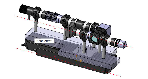
Figure 2 shows a real example of Abbe offset and error found in a microscopy instrument. In figure 2, the optical axis (the motion axis) has an offset (not coincident) with the encoder axis (measurement axis) and cause Abbe error in measurement reading.

2. Sine and Cosine error

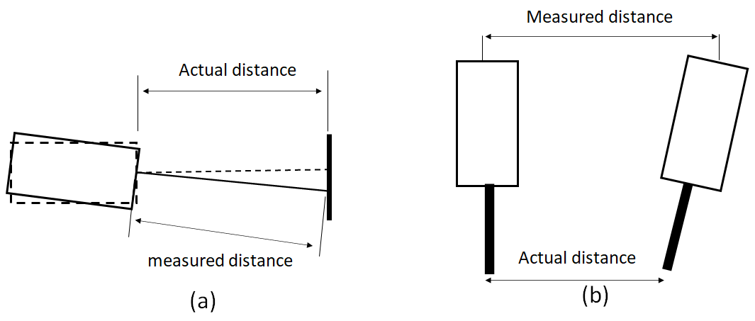
Sine and cosine errors are related to alignment imperfections in measurements. Figure 3 shows the illustration of both sine and cosine errors.

Sine error is similar to Abbe error. Meanwhile, cosine error is very common found in measurements using laser interferometry.

In figure 3, cosine error is due to the motion of an instrument (or of a measured part) is not perpendicular with the feature of a part measured by the instrument. Although, the measurement and motion axes of the instrument are coincident.

3. Datum (reference) error

Datum or reference error is a measurement error caused by incorrectly selecting a datum or reference in a measurement process. For example, in absolute distance measurement, a datum should be selected as a reference how far the distance is measured from. If the selected datum is incorrect, then the measured distance will be different with the actual distance.

4. Zeroing error

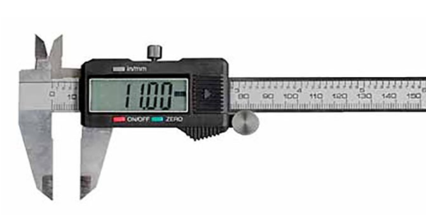
Zeroing error is due to a measurement reading is not set to zero. For example, a length measurement by using a digital calliper where the calliper’s digital reading is not set to zero. Figure 4 shows an example of a digital calliper having a digital reading.

If the digital reading does not start from zero value, for example 0.001mm, then there will be an offset error when reading a measurement from the digital reading as large as 0.001mm. This error is fix and systematic for all measurement with the digital calliper.

5. Misalignment error

Misalignments in measurement process will decrease the accuracy of measurements because, very often, misalignments cause sine or cosine errors. Misalignments can be caused by mistakes in measurement procedures or from geometry imperfections of measuring instruments.

Examples of misalignments from measurement procedures are the unprecise placement of a measured part, the mistakes in fixturing of a measured part and the incorrect selection of the measurement coordinate system measured by a coordinate measuring machines (CMMs).

Examples of misalignment from measuring instruments are the broken of the anvil surface of a Vernier calliper, the wear of the end surface of a calliper and misalignment of the measurement and motion axes of an instrument.

6. Structural error

Errors due to the structural imperfections (including geometry and configuration) of an instrument have large contributions to the total error on measurement results. A common method to reduce structural error is by manufacturing instruments’ components with very high accuracy, but, also with high production cost. This high production costs causes high instrument costs as well. Alternatively, software or numerical error compensation methods can be applied to reduce measurement errors originated form structural errors.

Some common structural errors are geometrical error, error due to deviations from kinematic design principle, error due to structure dynamics, thermal expansion, structural deformation, error due to deviations from symmetricity and error related to structural loop.

6.1. Geometrical error

One of the most important components on a measuring instrument is motion stage. This motion stage carry sensors used for measurement. Any errors related to this motion stage will directly contribute to measurement errors.

In most real cases, geometrical errors of instrument components are very small (in micrometre or even less). Although in micrometre scale, for measurement with accuracy at micrometre or higher level, these small errors are very significant and cause an instrument cannot be used for the measurement of parts with very tight tolerances.

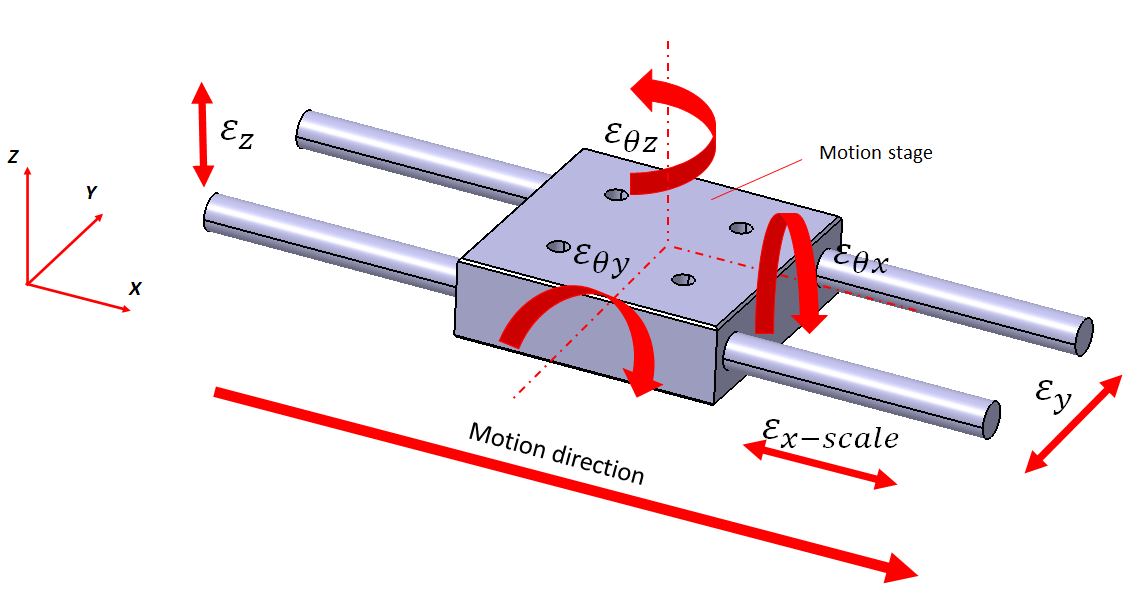
Figure 5 shows six degree-of-freedom (DoF) geometrical error of a single axis motion stage, in this case for x-direction motion. As shown in figure 5, each single axis motion will have 6 DoF errors: one scale error ($\epsilon _{x-scale}$), two straightness error ($\epsilon _{y}$ & $\epsilon _{z}$) and three rotational error ($\epsilon _{\theta x}$,$\epsilon _{\theta y}$,$\epsilon _{\theta z}$). Other direction motion axes will have the same 6DoF errors but only differ with respect to error directions.

In general, measuring instruments have three-axis motion stages that can move in x,y,z directions. With three axis motion stages, there will be a total of 21 DoF geometrical errors that are 18 errors for 6 DoF errors from each axis and three additional error for perpendicularly between the three axes.

Solutions to reduce these geometric errors are by manufacturing motion stages with high accuracy or by applying software (numerical) error compensations.

6.2. Error due to deviations from kinematic design principle

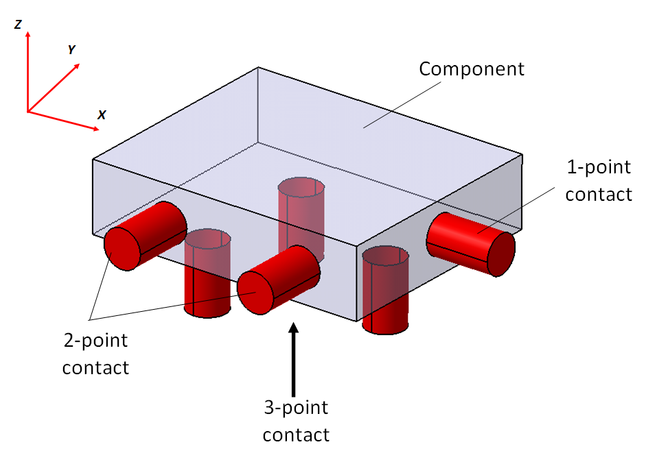
All measuring instruments, they are assembled from many components. Ideally, assembling two different components should satisfy the rule of 3-2-1 kinematic constraint as shown in figure 6.

In kinematic configuration, assembled parts will be sufficiently constrained without any residual stresses. Any deviations from kinematic constraint will cause additional stresses to components and cause deformation to components. Geometrical deviation on components will cause measurement errors on an instrument.

6.3. Error due to structure dynamics

Structural dynamics will be translated into vibration when performing measurements. Vibration on measurements is from two sources: the structure of an instrument and from environment.

For sensitive measurements, such as measurement with laser interferometers or areal optical surface topography measuring instruments based on interference methods, any low-level vibrations will degrade the accuracy of measurement results.

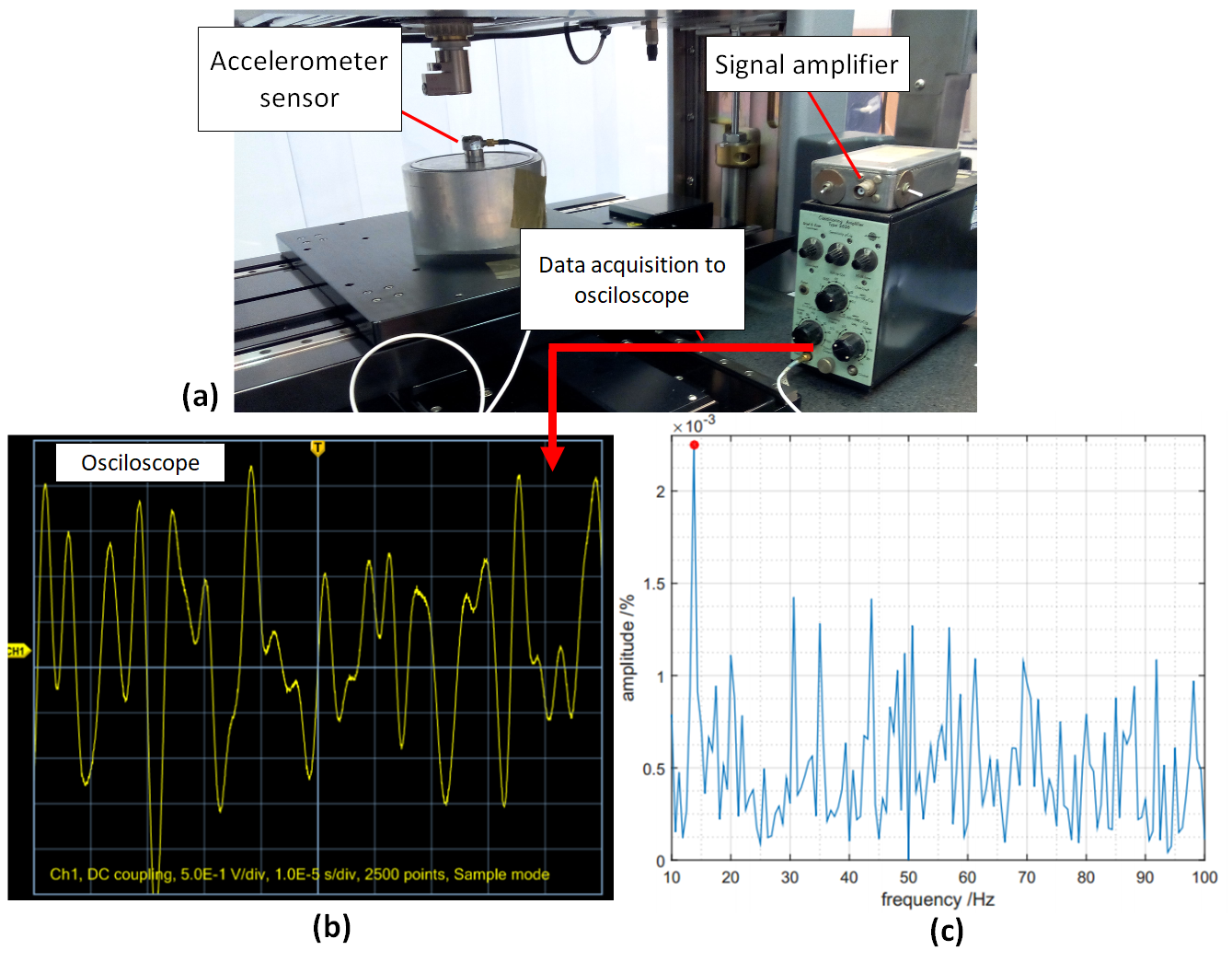
Figure 7 shows an example of vibration caused mainly from instrument structures and environment. In figure 7, an accelerometer sensor is placed on the table of an optical measuring instrument. As can be observed from figure 7, vibrations cause the instrument table to periodically move in vertical direction. This periodic motion will significantly reduce the accuracy of measurements, for example step height measurements at micrometre level.

6.4. Thermal expansion

For dimensional and geometrical measurement, the standard temperature (parts, instruments and environment) should be $20^{\circ}$C. Any deviations from this standard temperature when performing measurements will cause errors due to part and instrument material expansions.

Any parts and instruments are made from materials that have specific coefficient of thermal expansions. Any measurements carried out at $>20^{\circ}$C will cause parts and instruments having some degree of expansions. Meanwhile, any measurements carried out at $<20^{\circ}$C will cause parts and instruments having some degree of shrinkage.

Geometrical expansion and shrinkage of parts and instruments’ components will directly translated to measurement errors.

6.5. Structural deformation

Any components that are given loads will have some degree of compression. This compression will cause elastic deformations on the components. At minimum, the load is caused by the weight of the components themselves.

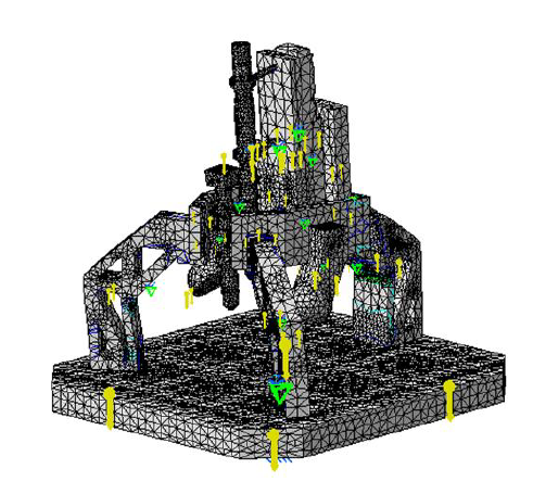
Since elastic deformations can be predicted, this deformation should be modelled and compensated when processing measurement results to reduce measurement errors. One common method to model and estimate elastic deformation is by performing finite element analyses (FEA).

Figure 8 shows an example of FEA of an instrument to estimate its elastic deformation. As can be seen from figure 8, the weight of the instrument itself can cause elastic deformation, at micrometre level, due to gravity.

6.6. Error due to deviations from symmetricity

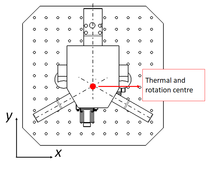
A symmetrical design has advantages that the design can reduce errors due to expansion or some degree of geometrical deformations on the parts constituting an instrument. Some advantages of symmetrical designs are having evenly distributed loads to reduce deformations concentrated at specific area and the same centre location for both thermal and rotation.

Figure 9 shows the benefit of having a symmetrical design. When the centre of thermal and rotation is at the same point, any thermal expansion to the geometry of the symmetrical design will have very small (if not zero) geometrical error due to rotation deformations.

6.7. Error related to structural loop

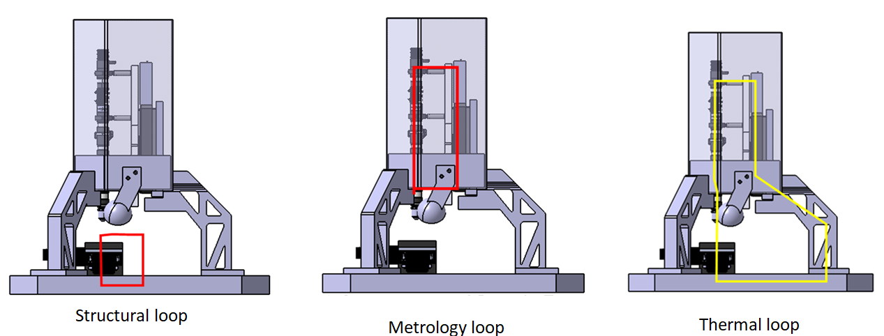
In any measuring instruments, there are three force loops act on the instruments. The force loops are structural, metrology and thermal loops. These three loops are shown in figure 10.

Ideally, these three force loops should be decoupled each other so that any geometry-related errors in a loop will not affect or be amplified to other loops. For example, the effect of errors on measurement results due to part deformation or expansion will be minimised.

Structural loop is a loop of forces via components that define relative positions between two objects, for example between a stylus tip and a measured part. Thermal loop is the loop of forces that defines the relative position between two objects (like structural loop) and is affected by thermal expansion of the components involved in the thermal loop. Metrology loop is a loop that pass components that read displacements, for example, a loop that goes through the encoder of an instrument.

7. Control error

Almost all high accuracy measuring instruments use error compensation methods, either hardware or software or both compensation methods. There are two types of error compensation: off-line and on-line.

Off-line error compensation can be applied to reduce systematic errors. These systematic errors can be modelled and quantified and predicted off-line. One way to quantify systematic errors, such as geometrical errors, is by performing a calibration process, for example using a laser interferometer.

Meanwhile, on-line error compensation can be applied to reduce random errors. On-line error compensation is implemented by using a real-time and close-loop control method. Real time and close-loop control are a control method that read the actual position of a motion stage at that moment in time and send feedback to the controller of a system to correct the actual position of the motion stage according to a commanded or desired position.

Implementing a real-time and close-loop control is difficult. For micrometre or higher level accuracy, the dynamics of an instrument and any other 2^nd or higher degree of non-linear errors should be modelled and taken into account when processing feedback data from sensor and adjusting position in real time.

8. Error due to surface roughness

The condition of part surfaces to be measured will affect the accuracy of dimensional and geometrical measurements, especially for measurement at micrometre- to nanometre-scale. The accuracy of general CMMs used for dimensional and geometrical measurements is high enough to detect roughness on a measured surface up to a certain degree.

Moreover, surface roughness will significantly affect the measurement of optical instruments, such as microscopy measurements. Because, light reflections, use to extract distance information, from surface roughness to the sensor of the optical instruments will vary following the degree of the roughness.

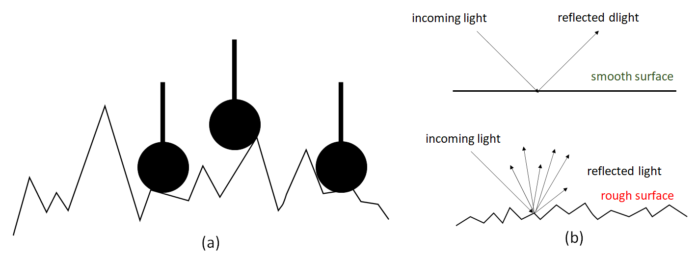
The illustrations of the effect of surface roughness on the measurement with contact (stylus) and non-contact (optical) instruments is shown in figure 11. In figure 11a, a micro stylus measures a flat surface. Because the “flat” surface has some degree of roughness, the stylus can read the roughness and will decrease the accuracy of flatness measurement on the surface.

In figure 11b, the effect of surface roughness on the measurements by using non-contact (optical) instruments is shown. As can be seen from figure 11b, the surface roughness cause the reflection of incoming light to spread in many different directions instead of one direction as in the case of a smooth surface.

9. Error due to dirt and dust

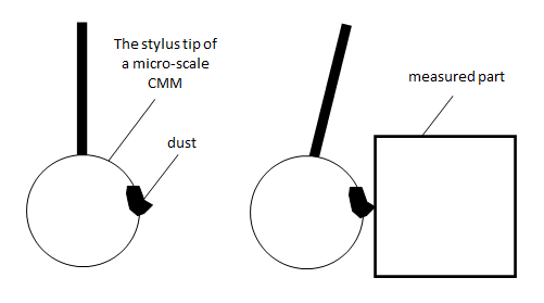
The accuracy of dimensional and geometrical measurements at micrometre- to nanometre-scale can be negatively affected by dust. Figure 12 shows the illustration of the effect of dust on dimensional and geometrical measurement accuracy.

In figure 12, dust will falsely trigger the stylus as detecting a surface. Since the detected surface is not correct, the measurement results, for example flatness and perpendicularity, will deviate from an actual value where the dust does not exist.

10. Non-technical error

Non-technical error is caused by the mistakes of operators who perform measurements with specific instruments. The most common types of non-technical measurement error are reading error and parallax error. To avoid these errors, good trainings for operator should be carried out.

Reading error is an error due to an operator incorrectly read measurement results from an instrument. For example, mistakes on reading the scale of micrometre. To avoid this mistakes, digital-based measurement readings can be implemented on the micrometre measuring instruments.

Parallax error is an error due to the view of an operator, who is reading a measurement result, is not perpendicular to the reading scale of a measuring instrument. This error very often found on instruments with line scales, such as ruler, calliper and micrometre. Also, this error can be caused by the use of eyeglasses by an operator. The glasses can cause reflections of light coming to the operator’ eyes.

Conclusion

There are many types of measurement error in dimensional and geometrical measurements. These types of error will contribute to the measurement uncertainty of measurement results and reduce the accuracy and precision of our measurements.

We need to understand these errors, especially what cause those errors, and avoid them when setting up, performing and reading measurements.

We sell all the source files, EXE file, include and LIB files as well as documentation of ellipse fitting by using C/C++, Qt framework, Eigen and OpenCV libraries in this link.

We sell tutorials (containing PDF files, MATLAB scripts and CAD files) about 3D tolerance stack-up analysis based on statistical method (Monte-Carlo/MC Simulation).