Applied programming

TUTORIAL: PYTHON for fitting Gaussian distribution on data

In this post, we will present a step-by-step tutorial on how to fit a Gaussian distribution curve on data by using Python programming language. This tutorial can be extended to fit other statistical distributions on data.

Wahyudin Syam

Jun 7, 2022 • 7 min read

The fitting of Gaussian distribution on data is very useful in research and development activities in all disciplines, including engineering, natural and social sciences as well as medicine.

A brief introduction about Gaussian distribution is given as refreshment about Gaussian distribution.

Let us go into the tutorial details!

Python Data Science Handbook: Essential Tools for Working with Data – A practical reference book in Python for breadth of computational and statistical methods that are central to data-intensive science, research, and discovery.

Gaussian (Normal) distribution: a short introduction

Random variable is defined as a real variable that is drawn or obtained from a random test or random distribution where the test values are within a specific sample set.

There are two types of random variables:

Continuous random variable
Discrete random variable

Continuous random variable is a random variable that has a value within a real interval either limited or unlimited.

Meanwhile, discrete variable is a random variable that has a value within a limited integer (finite) interval. Note that for discrete variable, the value is always within a finite limit.

Gaussian distribution is for continuous random variables. This distribution is the most well-known statistical distribution.

Gaussian distribution has been studied long time ago from the 18th century and is already well-understood, for example its properties.

In addition, many natural phenomena have distributions that like or follow Gaussian distribution. That is, many natural phenomena can be fit with Gaussian distribution to represent the property of the phenomena.

The probability density function (PDF) of Gaussian distribution is formulated as:

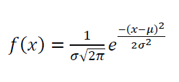
Where $- \infty \leq x \leq \infty , - \infty \leq \mu \leq \infty , \sigma > 0$. $\sigma ^{2}$ is the variance of the distribution and $\mu$ is the mean or average of the distribution.

The variable:

can be considered as a constant $C$.

NOTE that we can change the equation (1) into other statistical distribution functions to fit their distribution curves

PDF of a random variable $X$ is a mathematical function that describes the probability of a continuous variable $X$ drawn from a continuous statistical distribution, for example Gaussian, Exponential and Gamma distributions.

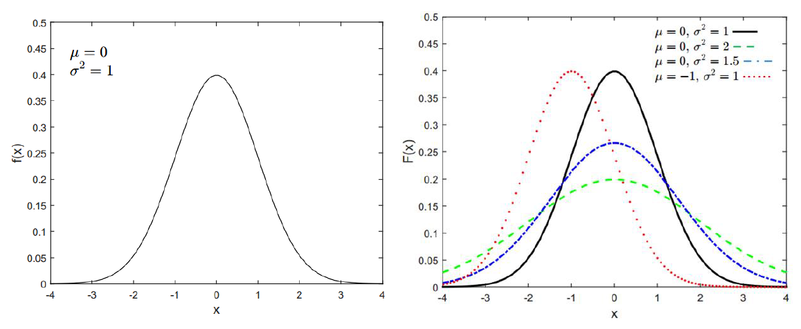
Gaussian distribution has a bell-shape curve. Figure 1 shows examples of Gaussian distribution curves or Gaussian probability density function (PDF).

Figure 1: Examples of different Gaussian curves (PDF) with different parameters. (left) is the basic Gaussian distribution curve (PDF) with mean = 0 and variance = 1 and (right) different types of Gaussian curve (PDF).

Python for Data Analysis: Data Wrangling with Pandas, Numpy, and Ipython – A book that provides comprehensive guides for manipulating, processing, cleaning, and crunching datasets in Python.

Step-by-step tutorial: Fitting Gaussian distribution to data with Python

The step-by-step tutorial for the Gaussian fitting by using Python programming language is as follow:

1. Import Python libraries

The first step is that we need to import libraries required for the Python program. We use “Numpy” library for matrix manipulation, “Panda” library for easy reading of files, “matplotlib” for plotting and “Scipy” library for least-square optimisation process.

import numpy as np
import matplotlib.pyplot as plt
import seaborn as sns

import pandas as pd

from scipy import stats
from scipy.optimize import curve_fit
from scipy import asarray as ar,exp

The most important library is “Scipy.optimize” for the least square fitting process via “curve_fit” function.

from scipy.optimize import curve_fit

2. Data reading

The next is to read the data from a file. The file can be an excel file, csv file or text file or any other files. In this case, we use text file to read the data from.

folder_path = 'Data.txt'
df_data = pd.read_csv(folder_path, sep="\t", header=None)

The pd.read_csv() has a parameter header set as None. Since our data in the text file does not contain any header, (only data), we use all the read value as data including the first row.

since all data manipulations such as vector and matrix are in “Numpy”, we convert the “panda dataframe” into “numpy” data format:

df_numpy=df_data.to_numpy(dtype ='float32')

Example of the data, in a text file opened by a notepad application, is as shown below:

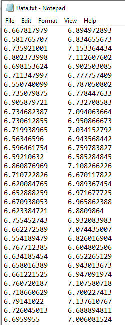
From the data above, after reading the text file, our matrix (Panda data frame) will have a size of nx2 matrix.

So, data reading is very flexible and we can do it in many ways…it is up to us.

3. Gaussian least-square fitting process

Since the data has two columns, in this case, we just want the first column of the data to fit the Gaussian distribution curve to.

Form these data, we then compute the histogram as:

x_data=df_numpy[:,0]

#plotting the histogram
hist, bin_edges = np.histogram(x_data)
hist=hist/sum(hist)

Figure 2 shows the calculated and plot histogram from the read data. From this histogram, we then fit the Gaussian distribution curve.

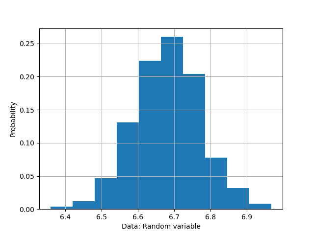
Figure 2: The histogram from the read data.

Then, we extract the histogram bin ($x$-axis) and values ($y$-axis) in figure 2. These two data are then used for fitting the Gaussian curve via a least-square optimisation. The codes to extract the histogram bin and probability values are as follows:

n = len(hist)
x_hist=np.zeros((n),dtype=float) 
for ii in range(n):
    x_hist[ii]=(bin_edges[ii+1]+bin_edges[ii])/2
    
y_hist=hist

Now, we have everything to perform the least-square fit on the histogram data (figure 2). The codes are below:

#Calculating the Gaussian PDF values given Gaussian parameters and random variable X
def gaus(X,C,X_mean,sigma):
    return C*exp(-(X-X_mean)**2/(2*sigma**2))

mean = sum(x_hist*y_hist)/sum(y_hist)                  
sigma = sum(y_hist*(x_hist-mean)**2)/sum(y_hist)

The least-square fitting process (optimisation) is as follow:

#Gaussian least-square fitting process
param_optimised,param_covariance_matrix = curve_fit(gaus,x_hist,y_hist,p0=[max(y_hist),mean,sigma],maxfev=5000)

The parameter to be optimised is $C$ (constant), $X_mean$ (the mean) and $sigma$ (the standard deviation). The optimisation above is basically minimising an objective function of:

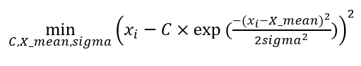
To fit other statistical distributions, we just need to change the equation (1) and adjust the parameter in the “def gaus(params)” function.

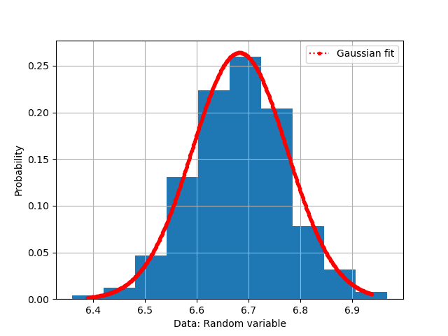
4. Plotting the Gaussian curve

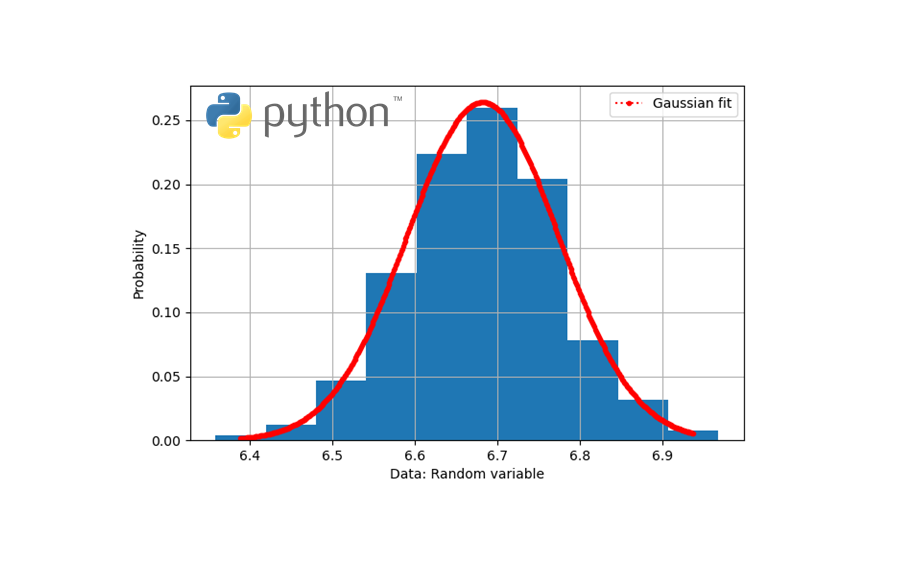
Finally, the plotting of the fit Gaussian curve as shown in figure 3 is as follow:

fig = plt.figure()
x_hist_2=np.linspace(np.min(x_hist),np.max(x_hist),500)
plt.plot(x_hist_2,gaus(x_hist_2,*param_optimised),'r.:',label='Gaussian fit')
plt.legend()

#Normalise the histogram values
weights = np.ones_like(x_data) / len(x_data)
plt.hist(x_data, weights=weights)

#setting the label,title and grid of the plot
plt.xlabel("Data: Random variable")
plt.ylabel("Probability")
plt.grid("on")
plt.show()

Figure 3: The Gaussian curve fit from the histogram of the read data.

Python codes for fitting Gaussian distribution

The full code to fit a Gaussian distribution to data is as follow:

# -*- coding: utf-8 -*-
"""
@author: wasy
"""
#STEP 1: IMPORT LIBRARIES ----------------------------------------------------
import numpy as np
import matplotlib.pyplot as plt
import seaborn as sns

import pandas as pd

from scipy import stats
from scipy.optimize import curve_fit
from scipy import asarray as ar,exp

#close all opened figure
plt.close("all")


#STEP 2: DATA READING---------------------------------------------------------
folder_path = 'Data.txt'
df_data = pd.read_csv(folder_path, sep="\t", header=None)

#Covert Panda dataframe to numpy
df_numpy=df_data.to_numpy(dtype ='float32')

#STEP 3: GAUSSIAN LEAST-SQUARE FITTING ---------------------------------------
x_data=df_numpy[:,0]

hist, bin_edges = np.histogram(x_data)
hist=hist/sum(hist)

n = len(hist)
x_hist=np.zeros((n),dtype=float) 
for ii in range(n):
    x_hist[ii]=(bin_edges[ii+1]+bin_edges[ii])/2
    
y_hist=hist
       
#Calculating the Gaussian PDF values given Gaussian parameters and random variable X
def gaus(X,C,X_mean,sigma):
    return C*exp(-(X-X_mean)**2/(2*sigma**2))

mean = sum(x_hist*y_hist)/sum(y_hist)                  
sigma = sum(y_hist*(x_hist-mean)**2)/sum(y_hist) 

#Gaussian least-square fitting process
param_optimised,param_covariance_matrix = curve_fit(gaus,x_hist,y_hist,p0=[max(y_hist),mean,sigma],maxfev=5000)

#print fit Gaussian parameters
print("Fit parameters: ")
print("=====================================================")
print("C = ", param_optimised[0], "+-",np.sqrt(param_covariance_matrix[0,0]))
print("X_mean =", param_optimised[1], "+-",np.sqrt(param_covariance_matrix[1,1]))
print("sigma = ", param_optimised[2], "+-",np.sqrt(param_covariance_matrix[2,2]))
print("\n")


#STEP 4: PLOTTING THE GAUSSIAN CURVE -----------------------------------------
fig = plt.figure()
x_hist_2=np.linspace(np.min(x_hist),np.max(x_hist),500)
plt.plot(x_hist_2,gaus(x_hist_2,*param_optimised),'r.:',label='Gaussian fit')
plt.legend()

#Normalise the histogram values
weights = np.ones_like(x_data) / len(x_data)
plt.hist(x_data, weights=weights)

#setting the label,title and grid of the plot
plt.xlabel("Data: Random variable")
plt.ylabel("Probability")
plt.grid("on")
plt.show()

Conclusion

In this post, a step-by-step tutorial on how to fit a Gaussian distribution curve on data has been presented. This technique is very useful for research and analysis in all fields from natural and social science, engineering to medicine.

This tutorial uses Python programming language. Beside free, this Python language is already well-known for scientific analysis. The source codes used in this tutorial are also presented and can be copied to use.

In addition, a brief introduction about Gaussian distribution is also given to refresh reader’s knowledge about Gaussian distribution as well as fundamental concept of probability density function.

This Gaussian fitting tutorial can be extended to fit other statistical distributions given the formula of distributions are known.

You may find some interesting items by shopping here.

We sell all the source files, EXE file, include and LIB files as well as documentation of ellipse fitting by using C/C++, Qt framework, Eigen and OpenCV libraries in this link.

We sell tutorials (containing PDF files, MATLAB scripts and CAD files) about 3D tolerance stack-up analysis based on statistical method (Monte-Carlo/MC Simulation).

Python Data Science Handbook: Essential Tools for Working with Data – A practical reference book in Python for breadth of computational and statistical methods that are central to data-intensive science, research, and discovery.