TUTORIAL: Visual Basic for Application (VBA) macro in Excel for Monte-Carlo Simulation
In this post, a hands-on tutorial of Visual Basic for Application (VBA) macro in Microsoft Excel for Monte-Carlo (MC) simulation is presented. MC simulation is a powerful tool to analyse and solve various scientific and engineering applications.
In this post, a hands-on tutorial of Visual Basic for Application (VBA) macro in Microsoft Excel for Monte-Carlo (MC) simulation is presented. MC simulation is a powerful tool to analyse and solve various scientific and engineering applications.
With VBA, powerful and useful MC simulations for various applications can be created.
Since VBA is a general-purpose programming, it can be used for many other useful applications for research and development in any scientific and engineering disciplines.
Visual Basic for Application (VBA) macro uses the implementation of Microsoft Visual Basic 6.0 programming language. The VBA can access Windows Application Programming Interface (API) to access windows functionality and to create customised user-generated functions or code to program or automate tasks in Microsoft office applications.
VBA macro is mostly used in Excel applications. However, it can also be used in other office applications such as Microsoft word and power point.
In this blog, a MC simulation application using VBA macro is applied for statistical tolerance stack-up analysis.
The tutorial will be shown from the simplest step (starting from how to show the developer ribbon in excel) until writing scripts to implement the MC simulation.
By the end of this post, readers can have hands-on knowledge of writing their own VBA script for various scientific and engineering analyses.
Let go into the details!
General view of the application of Monte-Carlo simulation using VBA macro-excel
In this tutorial, we will make a complete VBA macro application for statistical tolerance analysis with MC simulation.
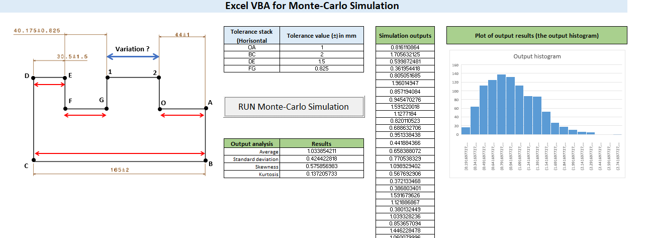
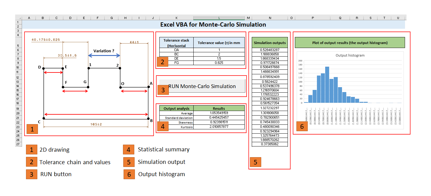
Figure 1 above shows the final layout of the VBA macro applications in Microsoft Excel. The application will contain the picture of the part and its tolerance chain, a table of the tolerance values involved in the tolerance chain, a command button to run the MC simulation by running the VBA macro script, a table showing a statistical summary of the simulation, a table showing the output for each MC simulation iteration and a histogram plot of the MC simulation outputs.
Before we go to the step-by-step tutorial, let us have a short discussion about tolerance stack-up analysis, presented in the next section.
(Readers that are familiar with tolerance stack-up analysis can directly skip the next chapter and jump to the chapter after)
Monte-Carlo (MC) simulation: an example to analyses 2D tolerance analysis
Tolerance stack-up analysis is a method used to evaluate the cumulative effect of allocated tolerances on parts constituting an assembly. The main goal is to assure that the functionality of an assembly can be delivered.
The tolerance analysis can estimate the total accumulated variation of the key characteristic (KC) of an assembly before the manufacturing of the parts constituting the assembly are performed. The analysis evaluates the tolerance values given to features on the parts.
In this case, we will perform statistical tolerance analysis.
In statistical tolerance analysis, the total accumulated variation (total variation) on the KC of an assembly is the root of a sum-squared addition of each tolerance in a tolerance chain.
Statistical tolerance analysis is formulated as:
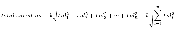
Where $k$ is a safety factor, $Tol_{i}$ is the tolerance value of the $i-th$ feature in a tolerance chain. If all parts are made in-house, the value of $k$ can be set to 1. Meanwhile, if some parts come from different manufacturers, the value of $k>1$, commonly assumed to be $k=1.2$. This $k$ factor is to consider additional part variations from other manufacturer.
Figure 2 below shows the tolerance chain and the tolerance values on a part that we want to analyse with MC simulations by using VBA macro in Excel. In figure 2, the KC that we want to evaluate the stack-up variation is the variations of the distance between point 1 and point 2.
Since the variation of the KC is in horisontal direction, only feature variations or feature tolerances in horisontal direction are considered.
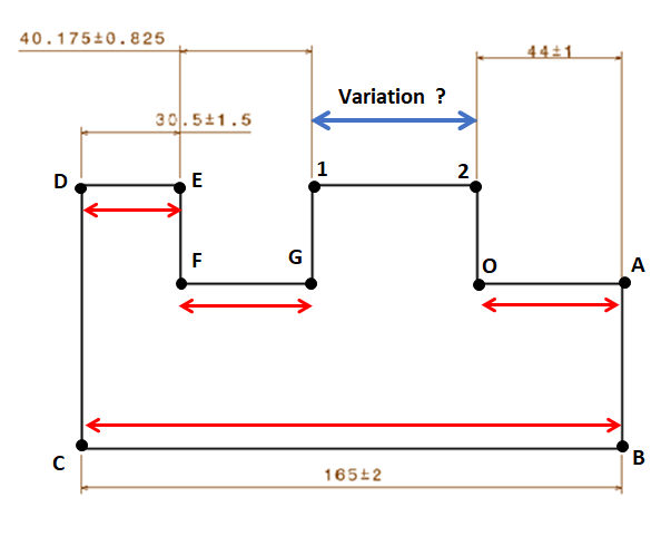
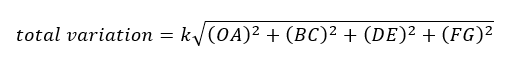
The total variation of the tolerance stack-up in figure 2 is formulated as:

Since only variations in horizontal direction are considered, the total variation formula can be shortened to be:
Let us go to the step-by-step tutorial in the next section.
Tutorial VBA macro-Excel for 2D tolerance analysis with Monte-Carlo (MC) simulations
We will do the step-by-step tutorial starting from how to show the developer ribbon in Microsoft Excel. Because, the developer ribbon, where we can access components for graphical user interface (GUI) components and the VBA macro editor (to write and edit VBA codes), is not shown by default.
1. Activating the Developer ribbon in Microsoft Excel
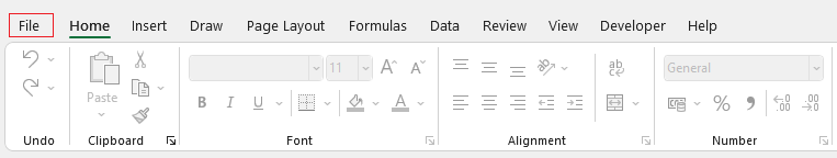
To show the developer ribbon, we can go to “file” and then press the “options” button.
Figure 3 below shows the “file” menu and figure 4 shows the “options” button in the file menu.
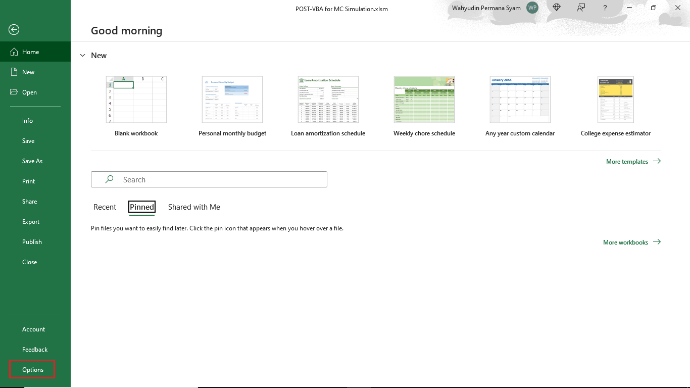
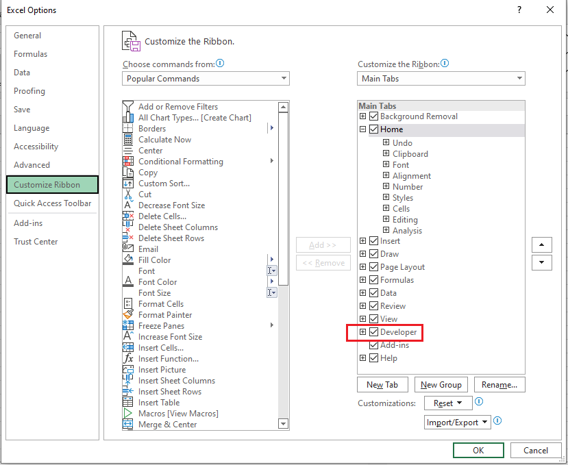
After pressing the “options” button, the “excel options” window will show up. Figure 5 shows the “excel options”.
From this “excel options” window, press the “customized ribbon” buttons and check the “Developer” that belongs to the “Main Tabs”. Figure 5 shows the process to check the “Developer” ribbon option.
By checking this “Developer” option, the “developer” Ribbon will show on the main menu. Figure 6 shows the “Developer” ribbon on the menu bar.
After we can activate the “Developer ribbon”, now we can start to design the Excel layout and add a command button for our MC simulation applications.
2. Creating the layout for the MC applications in Excel: command button, histogram, and input and output tables
Figure 7 shows the detailed layout of the MC applications that we will make. The layout consists of six elements.
The layout elements are:
- The 2D drawing and their assigned dimensional tolerance of the part or assembly we want to perform the tolerance stack-up analysis
- A table where we list all the involved tolerance in the tolerance chain, that are OA, BC, DE and FG. We fill the tolerance value for each dimension. This table is the input for the MC simulations.
- A command button when clicked or pressed, the MC simulation will run and put the results on the output table.
- A table that will show the output of the statistical summary of the simulation outputs. The statistical summaries are average, standard deviation, skewness and kurtosis.
- A table that will show an output from each simulation run. Since the simulation run will be set to 1000 runs, hence the table will contain 1000 rows to show the 1000 outputs.
- A graph to show the histogram of all simulation outputs (see layout component no 5 above). The histogram graph is set to have data from row = 6 to row = 6+1000 = 1006.
The layout can be straight forwardly created on the excel sheet.
It is important to note that the layout should follow the row and column position as shown in figure 7 above. Because the row and column determine the index when we access the data from a specific cell location by using the VBA code.
A special discussion will be presented related on how to make the command button to run the MC simulation (layout component no 3 above).
3. Adding command “Button” to add VBA macro code and start the MC simulation
We will discuss in detail for the layout component of the command button: how to create, set the properties and write the code that will be triggered by the click or pressed event of the button.
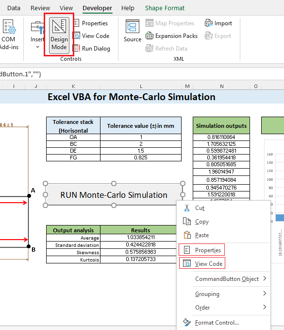
To create the button, we go to “Developer” ribbon and then click the “design mode” button.
When the “design mode” is activated, then we can insert the GUI components.
When we press the “insert” button, there will be several options for GUI components. Figure 8 shows the various types of GUI components and the one that we will use or select.
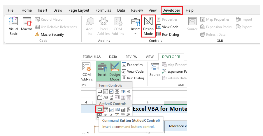
There are two groups of GUI components:
1. Form Controls
Form control is the old types of GUI components. They have an older look-and-feel window component. Also, we do not have flexibility to change many properties of the components, such as font and front colour. Also, to write a code for the event-handler, that is, what will happen when we press the button, we should make a function in the macro (see figure 9 below on how to open the VBA macro editor) and assign this VBA macro to the button. That is why we will use a better option, that is ActiveX Controls.
2. ActiveX Controls
ActiveX Controls have more flexibilities and look-and-feel compared to Form control components. These ActiveX control components have high flexibility to change their properties, such as font, colour and other graphical properties. In addition, it is very easy to create the event handler for the components.
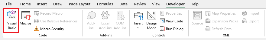
If we want to open the VBA macro editor (where we can code our VBA macro script), we can click the “Visual Basic” button inside the “Developer" ribbon as shown in figure 9 above.
Based on the above explanations of types of GUI Controls, we will use “command button (ActiveX Controls)” as shown in figure 8 above.
Then, we select the “command button (ActiveX Controls)” and drag to create the button as shown in figure 10 below.
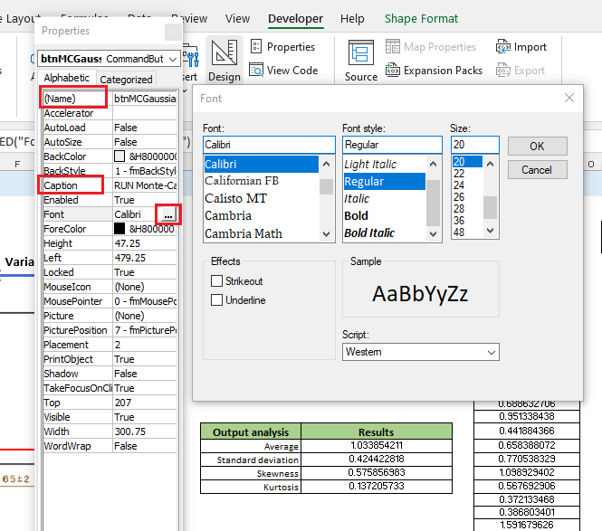
To set the properties and to add codes to program a task when the button is click by users (to run the MC simulations), we just need to right click the button (note: the “Design Mode” button should be active).
Figure 11 below shows the properties button when we select the “properties” upon right clicking the command button. In figure 11, we can see various properties that we can set to the button.
In this case, we set the “Object name”, “Caption” and “Font”.
“Object name” is to rename the button object that will be used to identify the button in the code.
“Caption” is to rename the text shown on the button in this case we set the value to be “RUN Monte-Carlo Simulation”.
“Font” is to set the fonts size, type, colour and other font-related properties.
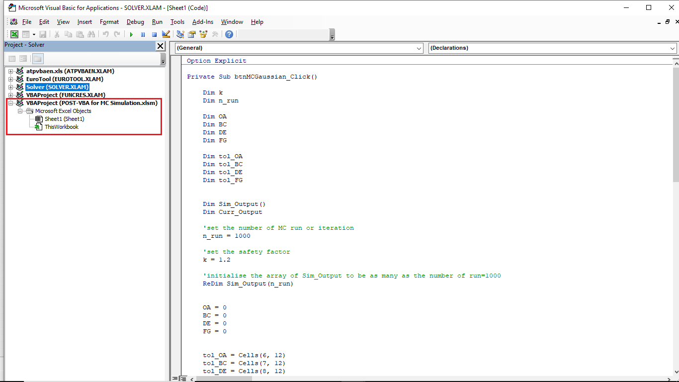
Figure 12 below shows the VBA macro editor where we can program the button to run the MC simulation when we click the button. We can right click the button and select “View Code” to open the editor and to write the VBA macro code.
The next step will discuss on how to make the code for the simulation and what is the meaning of the codes.
4. Writing the VBA macro code for the MC simulation
On the opened editor, we can start write the VBA macro code.
We will start with the:
Option explicitThe function of this “option explicit” is to make sure every variable should be declared before use. This imposed rule is very useful to make sure we define a variable before use so that we will minimise the risk of creating variables that we do not intend to make as variable.
The next step is to read the inputs from table in the layout element 2 (figure 7 above). The code to read the values form cells in the worksheet is as follow:
tol_OA = Cells(6, 12)
tol_BC = Cells(7, 12)
tol_DE = Cells(8, 12)
tol_FG = Cells(9, 12)
NOTE: if the input table locations in the layout is not the same as in figure 7 above, we should modify the Cell location accordingly.
The generation of random variable for Gaussian distribution uses the inverse transform method as follow:
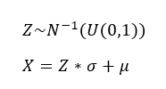
Where $Z$ is a random variable that is generated from $N^{-1}()$ which is the inverse of standard normal cumulative distribution, $U(0,1)$ is a random variable between 0 and 1 that is sampled from a uniform distribution, $\sigma $ is the standard deviation and $\mu$ is the average value, and $X$ is the generated random variable.
The standard deviation $\sigma $ is derived from the given tolerance value. Assuming that a tolerance value represents $3\sigma$, hence the $\sigma = TolVal/3$ where $TolVal$ is a given tolerance value.
The code to generate the random variables are as follow (just showing for OA dimension):
'OA dimension
Dim OA_input
MeanVal = OA
StDev = tol_OA / 3 'the tolerance is 3 sigma, hence to get one sigma, we devide the tolerance by 3
Z_Var = Application.WorksheetFunction.Norm_S_Inv(Rnd)
OA_input = Z_Var * StDev + MeanVal 'x=Z*sigma+mu
Finally, to calculate the tolerance stack-up on each simulation run, the code is as follow:
'total tolerance stack up (RSS) = sum-of-square
Dim SumSquare

SumSquare = OA_input * OA_input + BC_input * BC_input + DE_input * DE_input + FG_input * FG_input

Curr_Output = k * Application.WorksheetFunction.Power(SumSquare, 0.5)

Sim_Output(i) = Curr_Output
The VBA code for 2D tolerance analysis with Monte-Carlo (MC) simulations
The complete VBA macro codes (that handle the operation when we click the “RUN Monte-Carlo Simulation” button) used in this tutorial is shown as follow:
Option Explicit

Private Sub btnMCGaussian_Click()

    Dim k
    Dim n_run

    Dim OA
    Dim BC
    Dim DE
    Dim FG

    Dim tol_OA
    Dim tol_BC
    Dim tol_DE
    Dim tol_FG

    Dim Sim_Output()
    Dim Curr_Output

    'set the number of MC run or iteration
    n_run = 1000

    'set the safety factor
    k = 1.2

    'initialise the array of Sim_Output to be as many as the number of run=1000
    ReDim Sim_Output(n_run)

    OA = 0
    BC = 0
    DE = 0
    FG = 0

    tol_OA = Cells(6, 12)
    tol_BC = Cells(7, 12)
    tol_DE = Cells(8, 12)
    tol_FG = Cells(9, 12)

    'MsgBox tol_HI
    Dim MeanVal
    Dim StDev
    Dim Z_Var

    'Run the MC simulation with GAUSSIAN input
    Dim Start_Row
    Dim Index_Col

    'cell position to show the output for each MC simulation run
    Start_Row = 5
    Index_Col = 14

    Dim i

    For i = 1 To n_run

        'OA dimension
        Dim OA_input
        MeanVal = OA
        StDev = tol_OA / 3 'the tolerance is 3 sigma, hence to get one sigma, we devide the tolerance by 3
        Z_Var = Application.WorksheetFunction.Norm_S_Inv(Rnd)
        OA_input = Z_Var * StDev + MeanVal 'x=Z*sigma+mu

        'BC dimension
        Dim BC_input
        MeanVal = BC
        StDev = tol_BC / 3 'the tolerance is 3 sigma, hence to get one sigma, we devide the tolerance by 3
        Z_Var = Application.WorksheetFunction.Norm_S_Inv(Rnd)
        BC_input = Z_Var * StDev + MeanVal 'x=Z*sigma+mu

        'DE dimension
        Dim DE_input
        MeanVal = DE
        StDev = tol_DE / 3 'the tolerance is 3 sigma, hence to get one sigma, we devide the tolerance by 3
        Z_Var = Application.WorksheetFunction.Norm_S_Inv(Rnd)
        DE_input = Z_Var * StDev + MeanVal 'x=Z*sigma+mu

        'FG dimension
        Dim FG_input
        MeanVal = FG
        StDev = tol_FG / 3 'the tolerance is 3 sigma, hence to get one sigma, we devide the tolerance by 3
        Z_Var = Application.WorksheetFunction.Norm_S_Inv(Rnd)
        FG_input = Z_Var * StDev + MeanVal 'x=Z*sigma+mu


        'total tolerance stack up (RSS) = sum-of-square
        Dim SumSquare
        SumSquare = OA_input * OA_input + BC_input * BC_input + DE_input * DE_input + FG_input * FG_input
        Curr_Output = k * Application.WorksheetFunction.Power(SumSquare, 0.5)

        Sim_Output(i) = Curr_Output

        'write the current output to the cells
        Cells(Start_Row + i, Index_Col) = Curr_Output

    Next i

End Sub
Conclusion
In this post, a step-by-step tutorial on the use of VBA macro on Microsoft Excel has been presented and explained with a case study. The case study is to implement statistical tolerance analysis with Monte-Carlo (MC) simulations.
The tutorial explains a step-by-step procedure to develop the VBA macro applications, from activating the developer ribbon on the menu bar of the Excel to implementing the inverse transform to generate Gaussian random variables.
From these explanation and case study, readers can have a clear understanding and “how to” use VBA macro script in Excel to solve some of scientific and engineering calculations and analyses. The tutorial provides a hands-on experience to develop VBA macro applications on Excel.
We sell all the source files, EXE file, include and LIB files as well as documentation of ellipse fitting by using C/C++, Qt framework, Eigen and OpenCV libraries in this link.
We sell tutorials (containing PDF files, MATLAB scripts and CAD files) about 3D tolerance stack-up analysis based on statistical method (Monte-Carlo/MC Simulation).