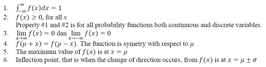
Continuous and discrete statistical distributions: Probability density/mass function, cumulative distribution function and the central limit theorem
In real world, all variables are random and the randomness is modelled by statistical distributions. In this post, various type of statistical distributions for both continuous and discrete random variables are explained.
In real world, all variables are random and the randomness is modelled by statistical distributions. In this post, various type of statistical distributions for both continuous and discrete random variables are explained.
As a starter, we will discuss the basic concept of probability density and mass functions as well as cumulative distribution functions.
In addition, the underlying concept of mean and variable of a statistical distribution is also explained.
By the end of this post, reader will understand the basic concept of statistical distributions and their types as well as understand the central limit theorem.
Probability density function, probability mass function and cumulative distribution function
Random variable
Random variable is defined as a real variable, let us call, X, that is drawn from a random experiment, let us call, e. This experiment e is within a sample set, let us call, S.
Since the results of the experiment e is not yet known, hence the value of variable X is also not yet known. The random variable X is a function that associates a real value of e within the sample set S from a random experiment.
Commonly, a random variable is notated as capital letter, such as X, Y, Z and $A$. the measured value from the random variable is commonly written as a lower case letter, such as x,y,z and $a$ for the random variables X,Y,Z and $A$.
For example, X is a random variable of a temperature. Hence, xis the measured value of X, for example x=25 degree C.
There are two types of random variables:
- Continuous variable: a variable that has a value with real interval and can have a finite or infinite limit. For example, length x = 2.567 mm and temperature t = 12.57 K.
- Discrete variable: a variable that has a value with finite (integer) interval and has a finite limit. For example, the number of defect components per 1000 components = 5 and the number of people in a queue = 15 people.
Probability function and cumulative distribution function
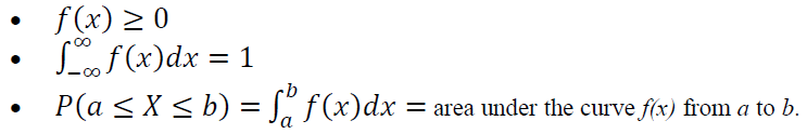
Probability function of a random variable X is a function that describe the probability of a variable X to be obtained.
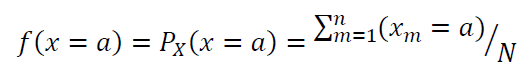
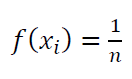
The notation for PDF is $f(x)$. Meanwhile, the notation for PDF is $F(x)$.
Based on the random variable types, probability distributions are also divided into two:
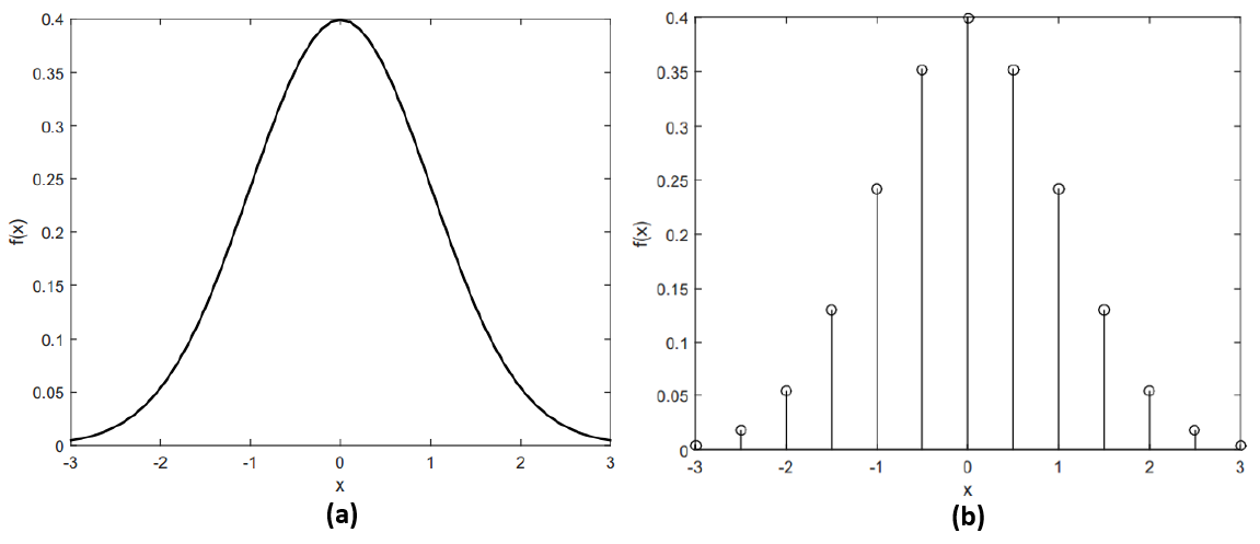
- Probability density function (PDF): the probability function of continuous random variable.
- Probability mass function (PMF): the probability function of discrete random variable.
Figure 1 shows an example of a PDF and PMF. In figure 1, we can observe that the PDF has real interval value (continuous) and PMF has finite interval values (discreet).
Discrete random variable
PMF is formulated as:
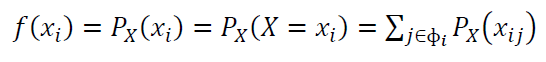
Where $X$ is a discrete random variable. $x_{i1}, x_{i2},…., x_{ik}$ represent the value of $X$ such that $H(x_{ij})=x_{i}$ for the set of index values $\Phi _{i}={j:j=1,2,…,s_{i}}$.
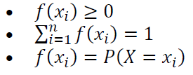
The properties of PMF are as follows:
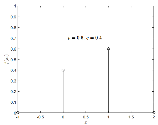
For discrete probability, we commonly say:
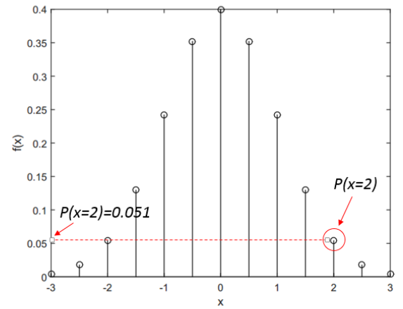
The probability of $X=a$ that is drawn from a sample set $S$, that is:
Where $a$ the discrete random variable from a sample set $S$ and $n$ the number of $a$ occurrences from $S$.
For example, a value of $a=2$ occurs from a discrete distribution $X$ so that the probability of $x=2$ or $P(x=2)$ is visually represented in figure 2 below.
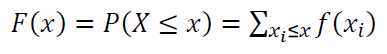
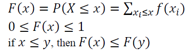
The cumulative distribution function (CDF) $F(x)$ of PMF is formulated as:
For discrete random variable, the properties of $F(x) are as follows:
Continuous random variable
PDF is formulated as:
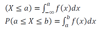
For continuous probability distribution, commonly we say as the probability of a value $X<a$ occurs from a sample set $S$ or the probability of a value $a<X<b$ occurs from a sample set $S$. These probabilities are formulated as:
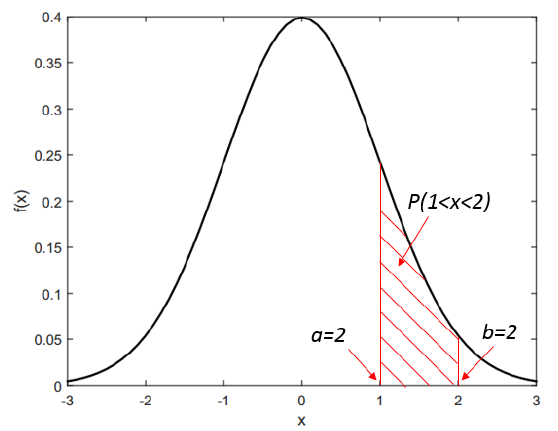
For example, the probability of a continuous random variable $X$ occurs with value between 1 and 2, that is $P(1<x<2)$ with, in this example, a Gaussian probability function is presented visually in figure 3.
The cumulative distribution function (CDF) $F(x)$ of PDF is formulated as:

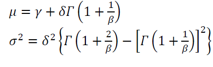
Statistical mean and variance
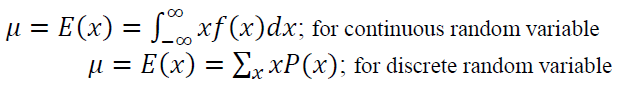
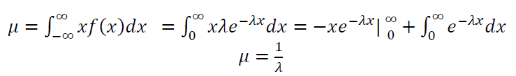
Mean or average $\mu$ is defined as a value that quantifies or describes the central tendency of a statistical probability distribution. Mean $\mu$ is expressed as the expected value of a random variable $E(x)$, that is the sample average from a long run repetition of a random variable.
Mean $\mu$ or expected value $E(x)$ is formulated as:
The other name of mean is the first moment of statistical distributions.
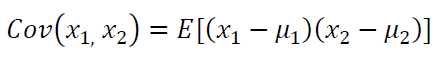
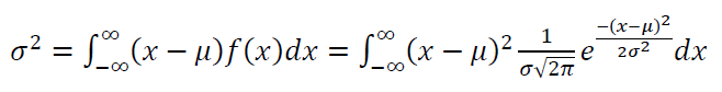
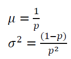
Variance $Var(x)=\sigma ^2$ is a value describing or quantifying the dispersion of statistical probability distributions. Variance $Var(x)=\sigma ^2$ is formulated as:
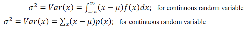
The Variance $Var(x)=\sigma ^2$ can also defined in term of expected value as:
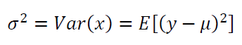
The square root of $\sigma ^2$, that is $\sigma$, is called standard deviation. The other name of variance is the second moment of statistical distributions.
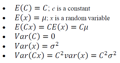
Important properties of expected values and variance
Important properties of expected values $E(x)$ and variance $Var(x)$ are as follows:
If there are two random variables, then:
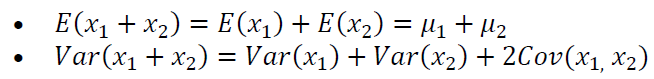
Where:
The properties of expected value $E(x)$ and variance $Var(x)$ mentioned above are very important and useful to know. One of the use of these properties is to derive the GUM formula to estimate the uncertainty of measurement results.
In the next sections, we will see many types of continuous and discrete statistical distributions. In addition, we will demystify the meaning of central limit theorem.
Continuous statistical distribution
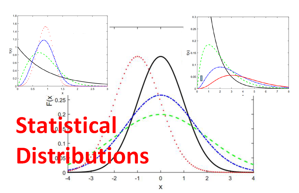
Types of continuous statistical distributions are: normal (Gaussian), uniform continuous, exponential, Gamma, Weibull and lognormal distributions.
Normal (Gaussian) distribution
Normal or Gaussian distribution is the most well-known statistical probability distribution. There are several reasons, such as, many nature entities follow this normal distribution and this distribution has been studied to understand the symmetrical pattern of measurement errors from the beginning of the 18th century.
Gauss is the first to publish this normal distribution in 1809. That is why distribution is also called Gaussian distribution.
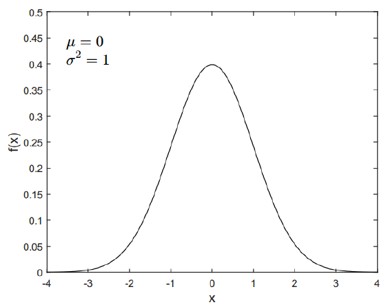
Normal distribution has a very unique symmetric shape like a “bell”. This type of distribution has a very important role in determining Type A measurement uncertainty in analysing other phenomena using regression and analysis of variance (ANOVA).
The PDF $f(x)$ of normal (Gaussian) distribution is formulated as follow:
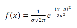
Where $-\infty \leq x \leq \infty , -\infty \leq \mu \leq \infty , \sigma >0 $. $\mu$ is the mean of the distribution and $\sigma ^2$ is the variance of the distribution.
A shortened notation to present normal distribution of a random variable $X$ is $X~N(\mu , \sigma ^2)$.
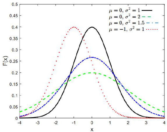
The PDF of normal distribution with mean = 0 and variance = 0 and with different values of mean and variance are presented in figure 4 and figure 5, respectively.
The properties of normal distribution are as follow:
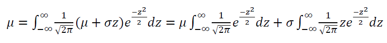
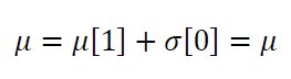
The mean $\mu$ of normal distribution is formulated as:
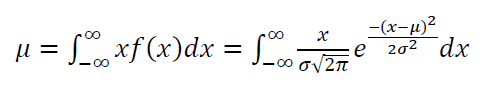
By using the variable:

Then we get:
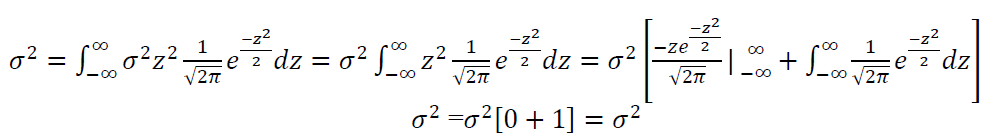
The variance $\sigma ^2$ of normal distribution is formulated as:
Similarly, by using the variable:

Then we get:
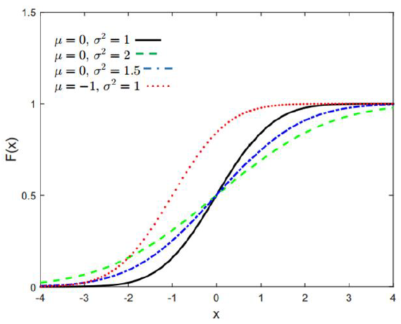
The CDF $F(x)$ of normal distribution is formulated as follow:
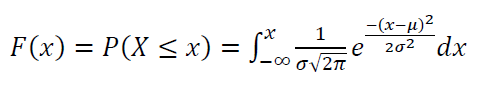
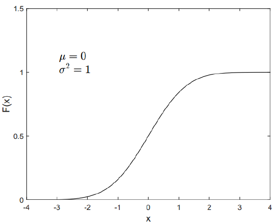
Figure 6 and 7 show some examples of normal distribution CDF with different mean and variance.
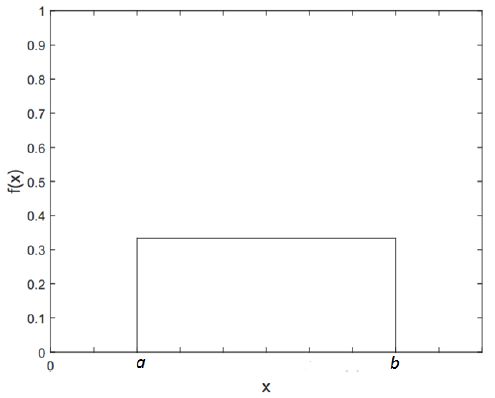
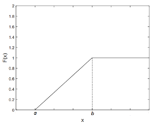
Uniform continuous distribution
Uniform distribution has an important application in measurement to determine the standard uncertainty from a calibration certificate or from a technical drawing (the tolerance).
The PDF of uniform distribution is:
Where $a$ and $b$ are the minimum and maximum value of the distribution.
The mean $\mu$ and variance $\sigma ^2$ of uniform distribution are formulated as:
The CDF of uniform distribution is:
Figure 8 and 9 show the PDF and CDF of continuous uniform distribution.
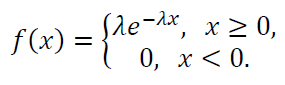
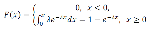
Exponential distribution
Exponential distribution is commonly used to model arrival time in computer simulation. The PDF of exponential distribution is as follow:
The CDF of exponential distribution is:
The mean $\mu$ of exponential distribution is:
The variance $\sigma ^2$ of exponential distribution is:
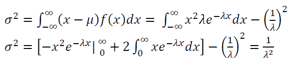
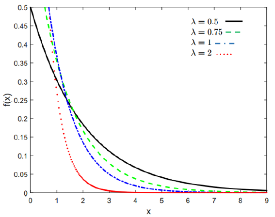
Figure 10 shows the PDF of exponential distribution with different means and variance.
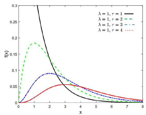
Gamma distribution
The PDF of Gamma distribution is defined as follow:
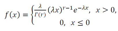
Where the parameter $\lambda >0$ and $r>0$. $\lambda$ is a scale parameter and $r$ is a shape parameter. $\Gamma (r)$ is a Gamma function = $(r-1)!$. Examples of the PDF of Gamma is shown in figure 11.
From figure 11, we can observed from the PDF of Gamma distribution above that exponential distribution is a special case of Gamma distribution where parameter $r=1$.
The mean $\mu$ and variance $\sigma ^2$ of Gamma distribution are formulated as:
The CDF of Gamma distribution is formulated as:
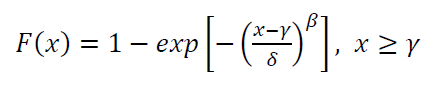
Weibull distribution
Weibull distribution is very common to be used to model the time-to-failure of mechanical and electrical systems.
The PDF of Weibull distribution is:
Where the parameter $\gamma$ is a location parameter with values $-\infty <\gamma <\infty $, $\delta$ is a scale parameter and $\beta$ is a shape parameter.
A unique feature of Weibull distribution is that, by adjusting its parameters, various types of probability distribution can be approximated.
Figure 12 shows Weibull distribution with various parameters.
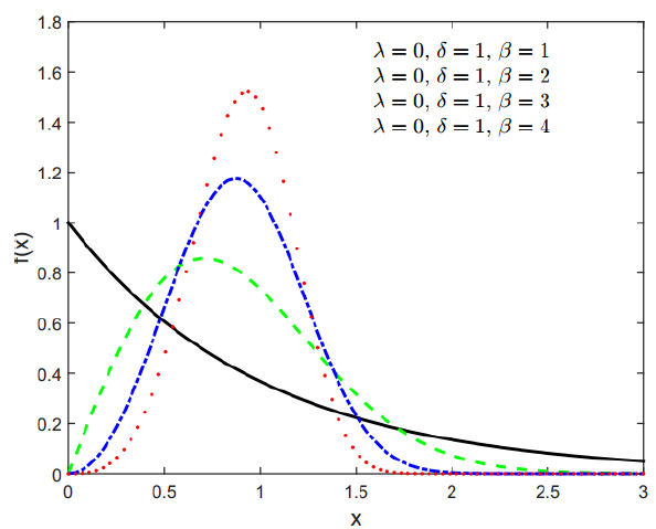
The mean $\mu$ and variance $\sigma ^2$ of Weibull distribution are formulated as:
The CDF of Weibull distribution is as follow:
Lognormal distribution
The PDF of lognormal distribution is formulated as:
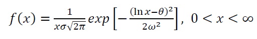
Where $\theta$ and $\omega$ are the lognormal parameters. Figure 13 shows lognormal distributions with different parameters.
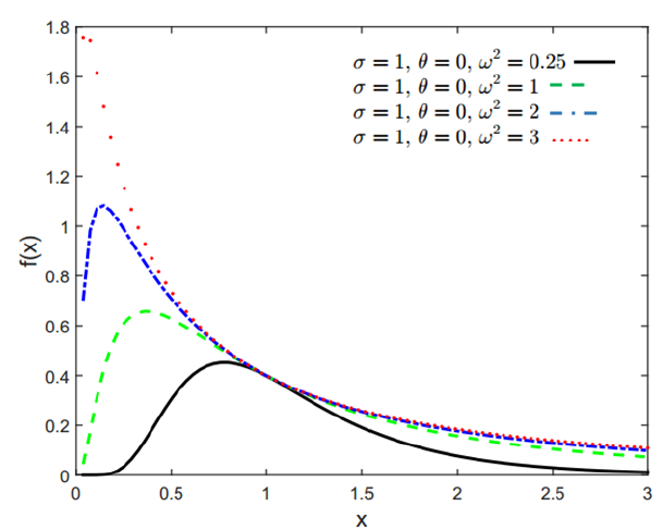
The mean $\mu$ and variance $\sigma ^2$ of lognormal distribution are formulated as:
Discrete statistical distribution
Types of discrete statistical distributions are: Bernoulli, uniform discrete, binomial, geometric and Poisson distributions.
The probability mass function PMF, that is the distribution function for discrete random variable, is visualised or presented as line diagram.
PMF of discrete variables is very useful to model qualitative measurement results that are commonly presented as integer value, for example, the colour code of a paint: 1 (black) and 0 (white). Other examples are the number of defective parts per batch and number of people arrival in a queue.
Bernoulli distribution
Bernoulli distribution has only two outputs. The PMF $f(x)$ of Bernoulli distribution is:
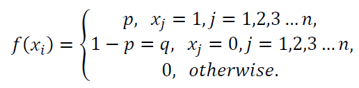
Figure 14 shows an example of the PMF of Bernoulli distribution.
The mean $\mu$ and variance $\sigma ^2$ of Bernoulli distribution are formulated as:

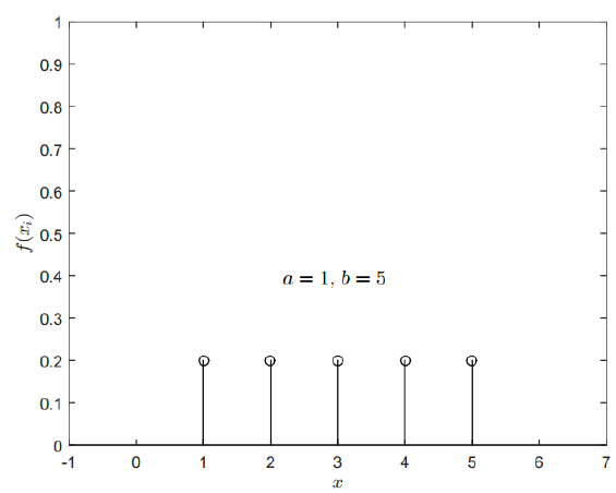
Uniform discrete distribution
The PMF of discrete uniform distribution is formulated as:
Where $n$ is the number of variable.
The PMF of discrete uniform distribution is shown in figure 15.
Meanwhile, the mean $\mu$ and variance $\sigma ^2$ of discrete uniform distribution are formulated as:
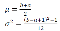
Where $a$ and $b$ are the minimum and maximum value of the random variable of discrete uniform distribution.
Binomial distribution
The PMF of binomial distribution is:
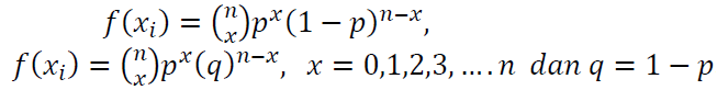
Where $n$ is the number of independent trials. Each trial only has two outputs, for example 0 and 1. $p$ is the output probability = 1 at each trial has values $0<p<1$.
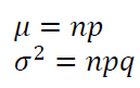
Figure 16 show the PMF of binomial distributions with different $n$ and $p$ values.
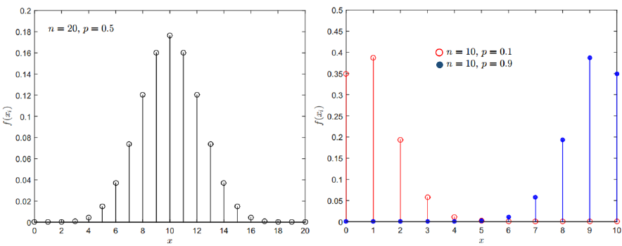
The mean $\mu$ and variance $\sigma ^2$ of binomial distribution are formulated as:
Geometric distribution
Geometric distribution describes numbers of trials of random variable $X$ until a certain output $A$ is obtained, for example the first occurrence of a failure or the first success.
The PMF of geometric distribution is:
Where $p$ is the distribution parameter with value $0<p<1$. Figure 17 show the PMF of binomial distributions.
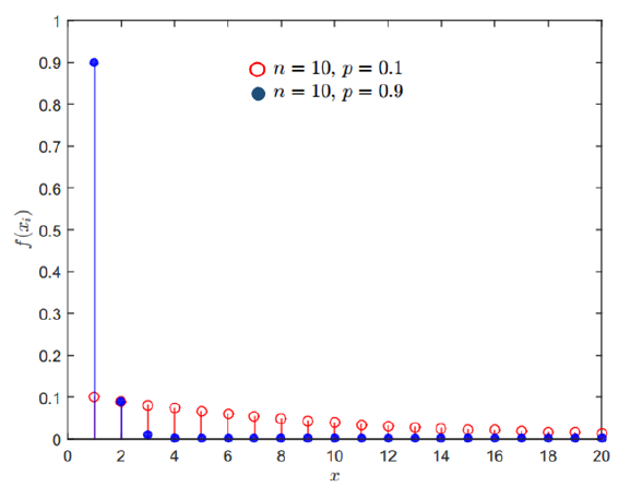
The mean $\mu$ and variance $\sigma ^2$ of geometric distribution are formulated as:
Poisson distribution
The PMF of Poisson distribution is:
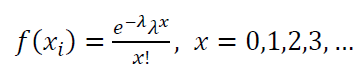
Where the parameter $\lambda$ has value $\lambda > 0$ and $\lambda=pn$. $n$ is the number of trials and $p$ the $p$-th event when an output with a certain value $A$ occurs.
The PMF of Poisson distribution with different values of $\lambda$ is shown in figure 18.
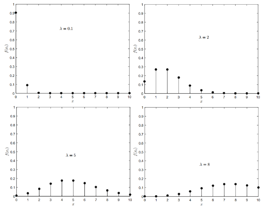
The PMF of Poisson distribution with different values of $\lambda$.
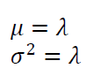
The mean $\mu$ and variance $\sigma ^2$ of Poisson distribution are formulated as:
The central limit theorem: Demystifying its meaning
In this section, we will demystify the true meaning of the central limit theorem.
Very common, people think that the central limit theorem says that any random variable if the number of trials or repetitions is very large toward infinite, they will follow normal distribution.
This is not correct!
Because, any events in nature have their own statistical distributions. For example, the distribution of dice output will always follow uniform distribution no matter how many times we repeat the dice experiments.
The true meaning of the central limit theorem is that when there are several or many random variables with different statistical distributions, if these variables are summed together, then the sum will follow normal distribution. In addition, the theory says that the arithmetic average of a random variable with a specific distribution, with high number of repetitions, the average will follow normal distribution.
The central limit theorem can be summarised mathematically as follow:
If $y_{1}, y_{2},…,y_{n}$ are series of $n$ trials and are random variables with $E(y_{i})=\mu$ and $V(y_{i})=\sigma ^2$ (both of these variables are finite numbers) and $x=y_{1}+ y_{2}+…+ y_{n}$, hence $Z_{n}$=

Has a normal distribution approximation $N(0,1)$ such that if $F_{n}(z)$ is a distribution function of $z_{n}$ and $\varphi(x)$ is the distribution function of random variables ~$N(0,1)$, hence:
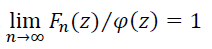
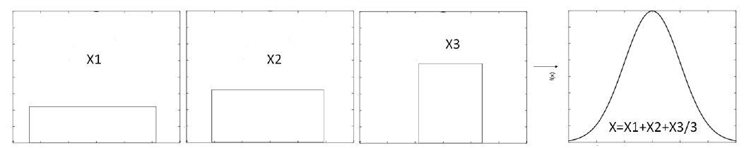
Figure 19 above shows the illustration of the central limit theorem based on the theory definition. In figure 19, when there are three random variables following uniform distributions with different parameters ($a$, %b% and number of trials), when the average of the summed three random variables is calculated, this average value will follow normal distribution.
The application of the central limit theorem on measurement, for example, is to estimate measurement uncertainty using Monte-Carle (MC) method. The MC method commonly has inputs of variables with different statistical distributions that model the random variables. The output of the MC simulation, with sufficiently large number of repetitions, will follow normal distribution.
Very common, the estimated uncertainty from an MC simulation will be calculated as the standard deviation of normal distribution of the simulation outputs.
Conclusion
In this post, the fundamental of statistical distribution and their mean and variance parameters are presented in detail.
Following the explanation of the distribution fundamental, various statistical distribution of continuous and discreet random variables are presented both their mathematical definition and their visual plots.
Finally, the true meaning of the central limit theorem is explained at the end of the post to correct common misunderstanding of the theory.
This knowledge of statistical distribution is essential to perform scientific analyses for research. For example, just to mention a few, to perform statistical data analyses and to estimate measurement uncertainty.
We sell all the source files, EXE file, include and LIB files as well as documentation of ellipse fitting by using C/C++, Qt framework, Eigen and OpenCV libraries in this link.
We sell tutorials (containing PDF files, MATLAB scripts and CAD files) about 3D tolerance stack-up analysis based on statistical method (Monte-Carlo/MC Simulation).
You may find some interesting items by shopping here.