Common problems in numerical computation: from data overflow, rounding error, poor conditioning to memory leak

In many modern science and engineering fields, numerical computation has an essential role to perform meaningful analyses. In numerical computation, many unexpected results occur due to errors related to digital computation instead of errors due to logic or model or formula errors.

There are at least two inherent problems in numerical computation using digital computers:

1. Very often, mathematical functions to compute are continuous. However, digital computers operate as a discrete system.
2. Commonly, numbers involved in our computation are infinite real numbers. However, our digital computers only process finite binary bits.

Hence, calculating functions or implementing numerical algorithms in digital computers have limitations.

In this post, at least six numerical computation errors are presented. The errors are data overflow and underflow, rounding error, poor conditioning, memory leak.

In addition, other important aspects in numerical computation, which are, processing speed and numerical optimisation are also discussed.

These errors are usually difficult to find as they are not obvious. By knowing these errors, we can at least reduce, or even prevent, the possibility to replicate these errors in our computational tasks.

1. Data overflow and underflow

One of fundamental aspects in computation with digital computers is to represent a real infinite number with finite number with bits (that have values either 0 or 1).

For example, a real number of $\phi=3.141592653589793… $ needs to be represented in term of finite bits. This representation is the fundamental computing error by using digital computers. This error is called approximation error.

Approximation error has an important role in intensive numerical computation with digital computers. Because, the error will be accumulated along the length of the computation chain and computation complexity.

There are two types of approximation errors: overflow and underflow errors. These two errors very often cause many numerical computational algorithm that are theoretically correct, but do not give correct or the same results from computation after implementations. This error is difficult to find, and sometimes, to resolve as well.

• Underflow error. This error occurs when a number close to zero is considered as zero.

This situation has a significant implication to computation results. For example, if we want to calculate $x=100000000000 \times 0.0000000001$, theoretically, the results should be $10$. However, in the real implementation, for example due to incorrect data type selection, a digital computer will consider the calculation as $100000000000 \times 0=0$. This result has a totally different result with the theoretical calculation.

Another example is when we want to calculate a division, for example, $x=1/0.0000000001$. If there is an underflow where $0.0000000001$ is considered as $0$. Hence the calculation becomes $1/0=\infty$ and causes the program to stop run or terminated.

Another more complex example is as follow. When we want to calculate a function:

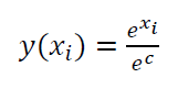
On the equation above, if the value of $c$ is a very large negative number hence the equation will have underflow, that is the denominator becomes 0. Hence, the results of the equation cannot be defined.

• Overflow error. This error occurs when a very large number is approximated as $\infty$. In a real situation, many digital computers will consider is as a not-a-number.

This overflow error has a significant implication to a calculation process. For example, $x=\frac{10000000000}{0.0000000001}=10^{20}$. If there is an overflow (perhaps, due to incorrect data type selection), hence the results will be $\infty$.

2. Rounding error

Rounding error is much related to approximation error that has been previously mentioned.

Rounding error also has significant effect to computations that have long and complex computing chains. The error can be caused by:

• Approximation errors due to digital computer limitations. For example, using an incorrect data type for a variable. For example, a variable that should store real number is set to have integer data type.
• Errors due to the programmer intentionally applied numerical rounding operation to data, for example using $round()$ and $ceil()$ in C/C++ language.

An example for this rounding errors is as follow. Suppose, we want to calculate an equation that has a short computational chain and is not complex as follow:

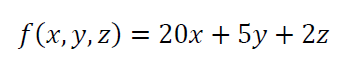
If the values of all variables in the equation above are $x=4.56, y=3.57, z=5.12$. Hence, the calculation result from the equation is $f(x,y,z)=119.29$. Meanwhile, if the variables in the equation above have rounded values of $x=4.5, y=3.5, z=5$, hence the calculation result is $f(x,y,z)=117.5$.

From the two computation results above, there is about 1.5% difference between the computation result with and without rounding. In this case, maybe, the difference is considered to be small.

However, when the computational chain and complexity become large (with the same variable values), for example:

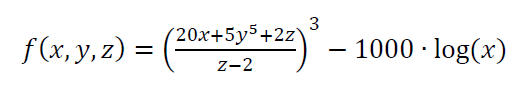
If the values of all variables in the equation above, as previous, are $x=4.56, y=3.57, z=5.12$, hence the calculation result is $f(x,y,z)=8.8 \times 10^{8}$. Meanwhile, when the variables value is rounded to $x=4.5, y=3.5, z=5$, hence the calculation results becomes $f(x,y,z)=7.5 \times 10^{7}$.

For the formula above, the difference of the calculation results between values with and without rounding is about 15.6%. In this example, it shows that the longer and more complex the formula, the larger the rounding error we get.

The rounding process in a numerical calculation also depends on what programming language used to perform the numerical computation. Hence, programmers should pay attention on what programming language they used to perform numerical calculations.

MATLAB programming language will round up a value that is ≥*.5. For example, a number of 4.5 will be 5 if it is rounded by MATLAB.

Meanwhile, PYTHON programming language will round down a value that is ≤ *.5. For example, the number 4.5 will be rounded to 4 by PYTHON.

One of practical recommendation to solve this rounding problem in the case where we want to test the results of a numerical computation is equal or not equal to 0, then it is better in the implementation, the 0 value is replaced with a variable, Let us say, epsilon $e$ that has a very small number, for example 0.0000001.

Hence the checking condition can be done with respect to this small epsilon value instead of with respect to 0 value. Of course the value of epsilon $e$ is based on computation goals.

3. Poor conditioning

Numerical conditioning is the measure of how large a function value changes with respect to a small change to its variables. It is similar to the definition of a “rate”.

A sensitive function, that is a function that will have a large change of value when its variables only have a small change of value, has a potential risk in numerical computation with digital computers. This condition is very often problematic in a condition such as inverse calculation.

This sensitive function is also called a function with poor conditioning property. Because, since this function will be drastically have a different value when its variables have only very small changes. Hence, when there is a rounding operation on the variables of the function, hence the value of the function will be significantly changed as well.

For an example, let say we have a function:

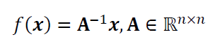
The above function has a conditioning value as:

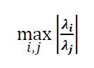
Where the value above is the ratio from the largest Eigen value $\lambda _{i}$ and the smallest Eigen value $\lambda _{j}$. Where this value is large, it means that the function has poor conditioning and is very sensitive with respect to the change of values of its variables.

Another example from a function with poor conditioning is a function that has one or more variables that have a very large exponent value. When there is a large change of value on the variable with very large exponent, then the value of the function will change significantly as well.

For example, a simple function $f(x)=x+5y=z^{40}$ is a function that has poor conditioning. Because, one of the function variable, that is $z$, has a very large exponent value that cause this variable is very sensitive with respect to a value change.

4. Memory leak

Memory leak in a software is a situation where a block of computer memory (random access memory/RAM) has been reserved for a variable (so that other variables cannot use the memory block).

But, after the variable that reserves the memory block is not used anymore, the reserved memory block is not freed. This un-freed memory cannot be used by other variables unless the computer is restarted.

The memory leak problem is very common in programming language with the capability of performing direct memory access, such as C/C++ programming language.

Despite the risk of memory leak, the advantage of the direct access memory capability is the memory management of a program can be customised and optimised to increase the processing speed of the software.

Memory leak problems will have a negative effect to the overall computer system and not only to a software that has the memory leaks.

For example, when we use a computer with 4 GB RAM and we run a program that is written with C language and blocks 8 kb memory for a variable and does not release or free the memory after use, this situation can affect the entire software system.

For example, if this variable is called from a function repeatedly and blocks 8kb each time the variable is used, then after 524288 iterations, the computer system will run out of memory. This run out of memory will affect the entire operating system of the computer and can cause the computer to stop operation and we will need to restart or reboot the computer.

In C programming language, to perform direct access memory, we can use $malloc()$ function. Hence, every variable that calls $malloc()$ function needs to free or release the memory blocked by the $maclloc()$ after using the variable. The memory release can be done by using $free()$ function. After calling $free()$ function, the memory block that has been reserved for the variable can be used again for other variable that need this memory block.

Another common problem with direct access memory in C language is segmentation fault problem. Segmentation fault is a situation where we are trying to access a memory block that is not available. A common example of segmentation fault is as follow. Suppose we have an array variable $*a$ as a pointer, when we want to access the element of array $a$ with $(*a+x)$, sometime we forget that the $x$ variable is not limited to a certain value and $a$ try to access a memory block that is not assigned for the $a$ variable.

5. Processing speed

The processing speed of a software significantly depends on what programming language used to make the software.

In general, the closer the programming language to machine language, the faster a software will run when the software is written by the language.

However, a programming language that closes to machine language is said to be low-level programming language, for example assembly language. Usually, the language will be harder for a human to directly understand and write codes compared to high-level languages, for example python and MATLAB.

The implementation of codes to make the same simple instructions with low-level language will be much longer than high-level languages.

For high-level language, that is a language that close to human natural language, the execution speed of this language is much slower than assembly language. However, this high-level language is easier to understand and require shorter line of codes than assembly language (low-level language).

At the moment, the famous high-level languages that are considered to have very high execution speed are C and FORTRAN. High-level languages that have high speed executions are usually based on compilation processes (based on compilers).

This is the reason why C and FORTRAN are usually used as baseline to compare the execution speed of other various high-level programming languages.

Examples of high-level languages that have slower execution speeds, compared to C ad FORTRAN, are Python, MATLAB, R, Ruby, PHP and others. Commonly, slow execution speed high-level languages are based on interpreter. The main advantages of these languages are that it is very easy to understand the languages and have high level abstractions so that codes can be written much shorter than C and FORTRAN versions.

Currently, Python is one of the most famous high-level languages based on interpreter. Python has a relatively faster execution time compared to other interpreter-based high-level language, such as MATLAB.

With Python, we can solve many scientific computation problem from basics to very advances. The availability of parallel computations makes the execution sped of Python can be reduced.

6. Numerical optimisation

Numerical optimisation is a process to estimate parameters of a function so that the value of the function is optimal. Optimal values can be minimum or maximum values depending on objectives.

Hence numerical optimisation can be divided into minimisation or maximisation processes.

In general, there are two types of solution for numerical optimisation that are direct solutions for close-form optimisation model or iterative solutions for open-form optimisation model.

Iteration process for numerical optimisation is an iterative calculation to calculate the value of an objective function, where on each iteration, the estimated parameters of the function is updated with new values. These new values are expected to improve the objective value on each iteration.

The iteration processes always require initial values or solutions to start the iteration process. These initial values can be based on random guesses, simple calculations or expert judgments.

Non-linear functions commonly require iteration solution processes.

A very common solution to convert the iteration solution for open-form model is by line arising the open-forms model into linear model. By this linearisation process, the open-form models can be converted into close-form and then can be solved with direct calculation solutions (without iteration).

The general form of numerical optimisation is as follow. If there is a set of inputs or parameters $\textbf{x}$ and a function $f(\textbf{x})$.

The other names of $\textbf{x}$ are decision variables or control variables or independent variables.

If we want to find a set of variables $\textbf{x} *, \textbf{x} * \in \textbf{x}$, so that $f(\textbf{x} *)$ where the value of $f(\textbf{x} *)$ is the optimal value of $f(\textbf{x} )$ (that can be a minimum or maximum value).

The general form of the optimisation is the optimisation of an objective function formulated as follow:

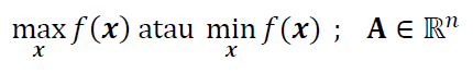
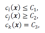
With or without one (or all) of these constraints:

The objective function (with or without constraints) is the function that we want to find the minimum or maximum value (depending on the case) of the function.

The constraints limit the solution space of the objective function. These constraint functions can be only one or all of them. The more the constraints function it has, the smaller the solution space will be.

For the optimisation of linear functions, the optimisation should has one or more constraints. Because, if linear functions do not have constraints, the solution space will be unbounded or infinite.

Meanwhile, for the optimisation of non-linear function, the optimisation has at least an inherent constraint from the function itself. For example, a non-linear function $f(x)=x^{2}+x+5$. This function has only one minimum function without any additional constraints.

Numerical optimisation is very common used to solve scientific and engineering problems. For examples, to find the best settings of a machine that has the least efficient fuel consumption and for geometric fittings from 3D point cloud data.

This geometric fittings need to minimise the orthogonal distance of each points with respect to the fitted geometry.

Numerical optimisation can be divided into three categories:

• Unconstrained problems

- Quadratic models. For example: $f(x)=\frac{1}{2} x^{2}$

- Non-linear but non-quadratic. For example: $f(x)=\frac{1}{4} x^{3}+2x$

• Linearly constrained problems

- Model with equality constraint

- Model with inequality constraint

• Non-linear problems with or without constraints

- Model with equality constraint

- Model with various types of constraints

As mentioned before, non-linear models require iterative solutions with initial solutions given. In geometrical measurements, these models are very common to associate point cloud to a nominal geometry.

For example, the fitting of point cloud to a nominal cylinder. After this fitting process, the cylinder geometry measurement can be performed, for example to find the cylinder diameter.

Conclusion

In this post, we have discussed the most common problems found in numerical computations with digital computers.

Numerical computation is very important in modern science and engineering and to solve complex problems.

These problems are due to the inherent working principle of digital computer that need to represent number in finite number of bits.

We have presented in details with examples how these problems can significantly affect the results of numerical computations. And, ways to prevent these problems are also presented.

We sell all the source files, EXE file, include and LIB files as well as documentation of ellipse fitting by using C/C++, Qt framework, Eigen and OpenCV libraries in this link.

We sell tutorials (containing PDF files, MATLAB scripts and CAD files) about 3D tolerance stack-up analysis based on statistical method (Monte-Carlo/MC Simulation).