Error compensation for coordinate measuring instrument: The mathematical model of 3-axis coordinate measuring machine (CMM)

The mathematical model of a measuring instrument is important for building the error compensation system for the instrument.

In this post, the mathematical model of a 3-axis coordinate measuring machine (CMM) and only consider kinematic errors is presented and discussed [1].

The 3-axis CMM has a FXYZ configuration. This FXYZ configuration is the most widely used CMM configuration in industry.

In this FXYZ configuration, a measured workpiece or part is fixed on a measurement table. Meanwhile, the probing system of the CMM can move relative to the workpiece or part in X,Y and Z axis or directions.

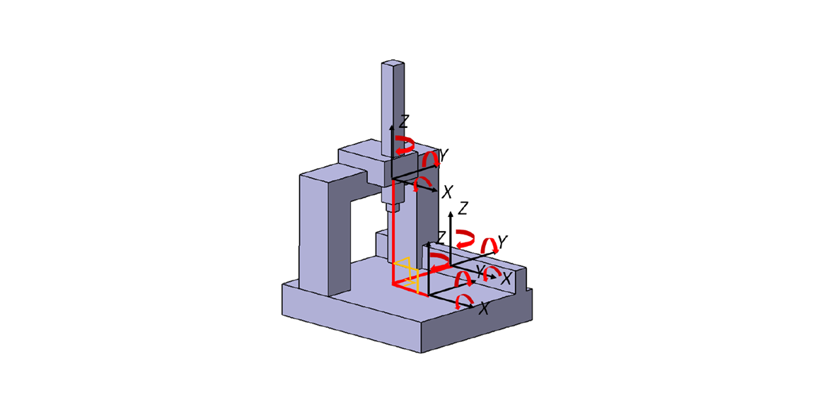
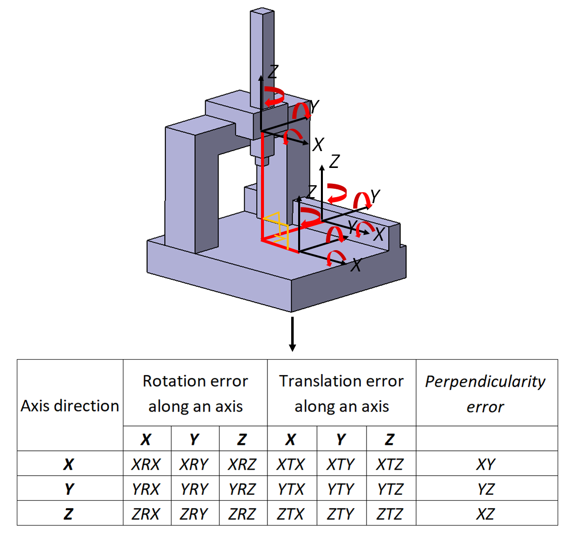
Any 3-axis CMMs, either with FXYZ configuration or with other configurations, have a total of 21 kinematic errors. Figure 1 below shows the 21 kinematic errors. These kinematic errors are obtained from 18 kinematic errors of the three axes and three perpendicularity errors between two axes from out of all the three-axis combinations.

The mathematical model of kinematic errors only considers geometrical errors on the components (due to machine process imperfections or defects) constituting a CMM and is called as “rigid-body” model. This “rigid body” model does not consider other errors, such as load error, thermal error and other errors. 

The main assumption of a “Rigid body” model is that this model considers that a CMM is very stiff such that no bending (or very little so that can be ignored) occurs due to internal (from the CMM components) and external loadings (from measured parts and fixturing systems).

With “Rigid body” model that only consider the kinematic errors of a CMM, it is reported that, with an implementation of error compensation based on “rigid body” model only, the accuracy of a FXYZ type CMM can be improved up to 10 times than when no error compensation is applied [1].

There are other mathematical models for various types of CMM configurations that consider other errors, such as thermos-mechanical error, load error, dynamical error, and motion control error [2].

READ MORE: Error compensation for coordinate measuring instrument: Steps and calibration instruments

Mathematical error model of a 3-axis coordinate measuring machine (CMM)

The “rigid body” mathematical model of a FXYZ type CMM is shown in figure 2 below. In figure 2, there are four independent coordinates, that are:

• The coordinate system on the CMM table $(O,X,Y,Z)$
• The coordinate system on the Y-axis or bridge $(O_{1},X_{1},Y_{1},Z_{1})$
• The coordinate system on the X-axis $(O_{2},X_{2},Y_{2},Z_{2})$
• The coordinate system on the Z-axis or ram $(O_{3},X_{3},Y_{3},Z_{3})$

The motion system configuration of the CMM is that the X-axis motion system is placed on the Y-axis motion system. Meanwhile, the Z-axis motion system is placed on the X-axis motion system.

The mathematical notations on the mathematical error model are as follows: variables represent the direction of axis motion and subscript represents the direction of errors. For example, $\delta _{x}(Y)$ is the straightness error on X-direction for Y-axis motion and $\varepsilon _{x}(Y)$ is the rotation error around x-axis for Y-axis motion.

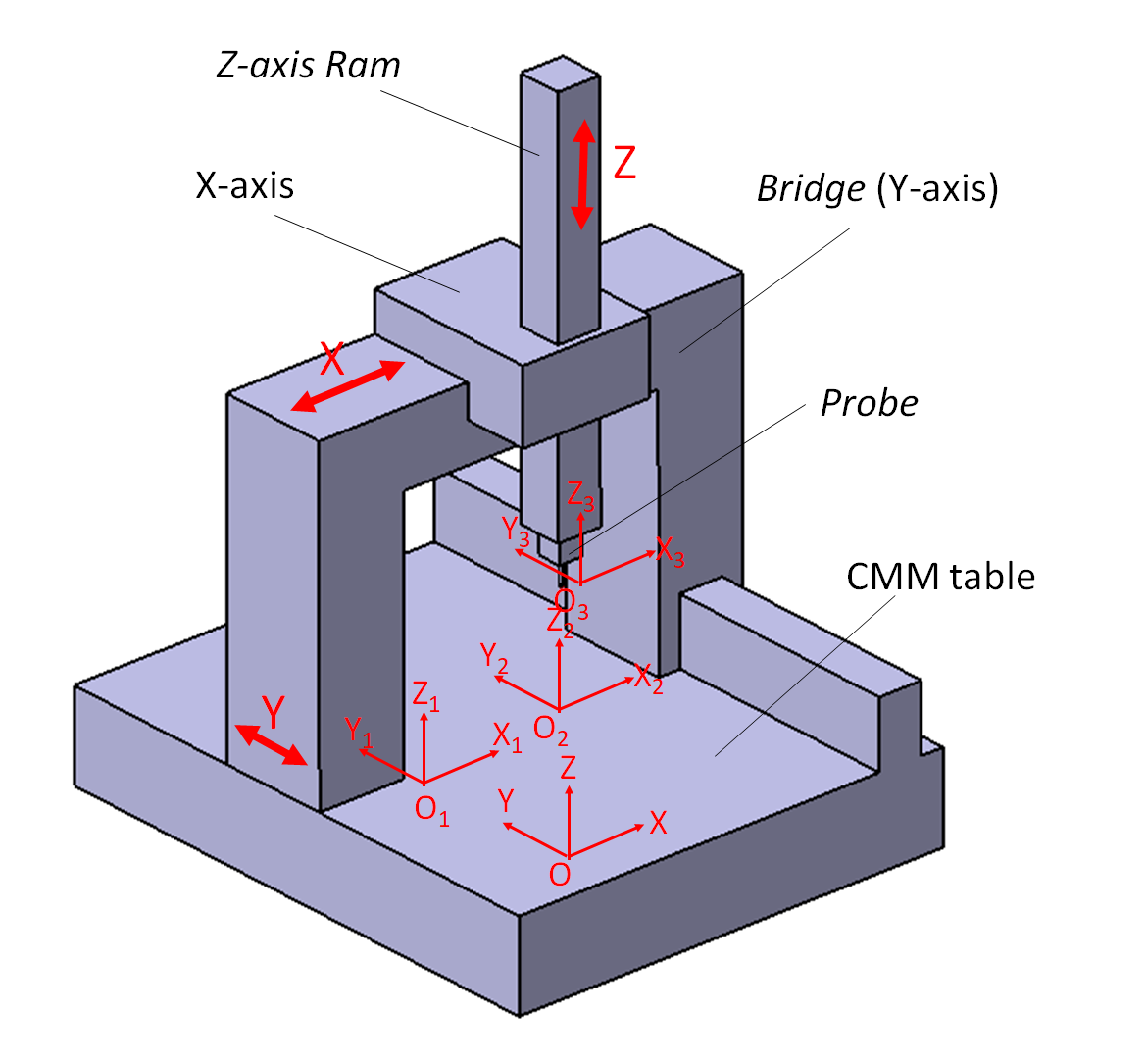
An Initial assumption is that all the four axes (explained above) are at the same origin (in initial condition). In another word, the initial position of the CMM probe is at the bottom front-corner on the CMM shown in figure 2 above.  

From figure 2, an initial motion to reach the position shown in figure 2 is started by moving the Y-axis. Hence, when the Y-axis or bridge move as many as Y distance, then the actual position of the coordinate system of the Y-axis (that is $O_{1}$) is represented by a vector as follow:

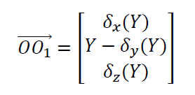
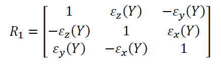
When the Y-axis moves, not only straightness error, but also there will be a rotational error on the Y-axis (bridge) with respect to the coordinate system of the CMM table. This rotational error can be represented as follow:

Also when the X-axis moves as many as X distance, then the coordinate transformation from $O_{1}$ to $O_{2}$ is formulated as:

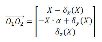
Where the angle $\alpha$ is the perpendicularity error between the X-axis and the Y-axis. Also when the Z-axis moves as many as Z, then the coordinate transformation from $O_{2}$ to $O_{3}$ is formulated as:

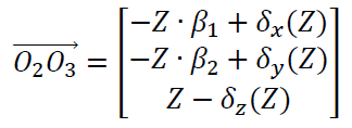
Where the angle $\beta _{1}$ and $\beta _{2}$ are the squareness errors between the Z-axis and the XY-plane.

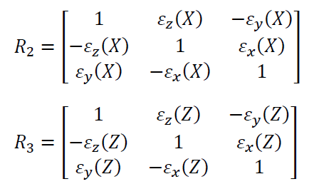
The rotational error for $O_{2}$ and $O_{3}$ are:

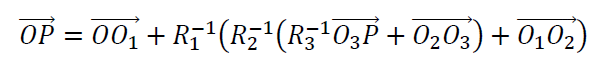
Point $P$ is defined as a point with coordinate $(X_{p},Y_{p},Z_{p})$ on the coordinate of the Z-axis/ram.

Then, the coordinate of point $P$ with respect to the coordinate system of the CMM table is $(X’,Y’,Z’)$ is determined as follow:

From the equation above, then the error function of a position $P$ is formulated as:

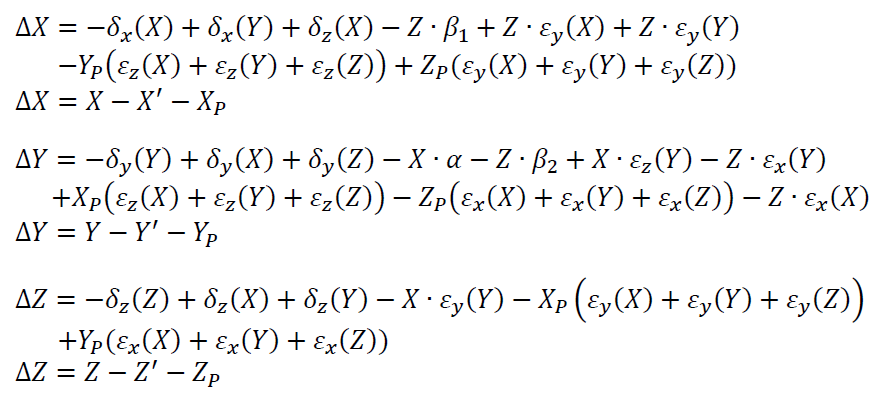
Where $\Delta X, \Delta Y, \Delta Z$ are the errors of a point $P$ in X,Y and Z direction. The value of $\Delta X, \Delta Y, \Delta Z$ are the errors that need to be compensated by the control system of the CMM for a commanded position.

Hence, if a position needs to be reached, the numerical control system will command a motion to the position after being compensated as many as $\Delta X, \Delta Y, \Delta Z$.

Very common, measurements with a laser interferometer system or measurements of calibrated artefacts are used to quantify the kinematic error components of CMMs.

READ MORE: Error compensation for coordinate measuring instrument: introduction and types

Conclusion

In this post, the mathematical model of 3-axes CMM has been discussed. The model follows an assumption of “rigid body” where only kinematic errors are considered. Other errors are not considered in this modelling.

From a report by [1], by only compensating these kinematic errors, a 10 times accuracy improvement can be obtained for a 3-axes CMM machine.

 Reference

[1] Zhang, G., Veale, R., Charlton, T., Borchardt, B. and Hocken, R., 1985. Error compensation of coordinate measuring machines. CIRP annals, 34(1), pp.445-448.

[2] Hocken, R.J. and Pereira, P.H. eds., 2016. Coordinate measuring machines and systems. CRC press.

You may find some interesting items by shopping here.