Metrology

Error compensation for coordinate measuring instrument: Steps and calibration instruments

For the implementation of error compensation on measuring instruments or machine tools, there are steps to follow, that are the reconstruction of an error map (via mathematical modelling via analytical or empirical methods) and the calibration process to quantify and characterise the error map.

Wahyudin Syam

Oct 28, 2023 • 10 min read

In the previous post, the reason on why error compensation is required and types of error compensation have been discussed. Mostly, error compensation focuses on correcting systematic errors.

Because, systematic errors are repeatable and can be modelled. However, random errors can also be compensated with a real-time error compensation only.

In this post, the steps to develop and implement error compensation methods on instruments with motion systems will be presented.

Reconstructing the mathematical model of errors: analytical and empirical methods

The reconstruction of an error map, representing the error on a certain position or location in the measuring volume or working volume of a machine, can be performed by using an analytical or empirical method.

An error map can only be reconstructed for systematic error [1].

There are conditions for systematic error to be able to be compensated:

The value of the systematic error of an instrument to be compensated should be significantly larger than the random error. That is, the instrument to be compensated should be “repeatable”.
The benefit of an error compensation implementation should justify the additional cost required to implement the error compensation.
The rate of spatial change of an error should be lower than the standard dimension interval used to quantify the error. That is, it is important to select an instrument to quantify the error. For example, whether to use continuous standard such as laser interferometer or to use discontinuous standard, such as ball bars, ball-plates and gauge block.
An instrument to be compensated for should have an absolute coordinate system. In addition, the repeatability of the absolute system should be lower than the spatial change rate of an error to be compensated.
The performance of a computer (such as computational speed, resolution, spatial frequency correction and others) and a servo as well as other required instruments should be enough to meet the demand of the processing of an error compensation implementation.
The error model of an instrument (the error map) should be available. This error map is a mathematical model of errors that relate error sources and the error they cause and to determine what parameters of the error map that need to be quantified via an experiment (calibration).

The mathematical model, based on analytical method, of an instrument depends on the type of errors that are considered when making the mathematical model [2].

Types of error on measuring instruments

Kinematic error

Kinematic error is defined as error that is originated from the geometrical imperfection of the components constituting the instrument due to variation of manufacturing processes. Besides, kinematic error can also be caused by configuration mistakes, for example misalignment between two axes. Kinematic error is the main error to be considered to reconstruct the mathematical model of an instrument.

Thermo-mechanical error

Thermo-mechanical error is caused by the dimensional expansion or shrinkage of the geometry of a component. This expansion and shrinkage are caused by temperature changes from inside and outside of the components. Any materials have a coefficient thermal expansion that indicates how large the material will expand or shrink proportionally with respect to temperature changes.

Load error

Load error is the deformation of components due to loads applied to the components. This error should be considered if the mathematical model of errors assumed for an instrument to model is as “non-rigid body”. This assumption is valid because any materials have a limited stiffness. This load error in certain situations can be higher than kinematic errors of components due to, for example, bending on components.

Dynamic error

Dynamic error is caused by the acceleration and deceleration of a motion system. The obvious effect of this motion is vibration on the components of the motion system. This vibration causes a small displacement of the components. Very often, to reduce this vibration, the speed of the motion system of an instrument is set low.

Motion control error

Motion control error is an error caused by faults from a control system. These faults can be from the software such as imperfect control algorithms or from hardware, such as actuator imperfections.

One of the advantages of mathematical error models based on analytical approaches is that an error quantification by calibration process only requires small number of quantifications at certain positions only. Because, from these small number of quantified errors, with the analytical model, the whole error map can be estimated.

With analytical approaches, the cost of calibration processes to quantify errors can be significantly reduced.

The main drawback of analytical error model is that the accuracy and effectiveness of the model significantly depends on the assumption of what error sources are relevant, for example, very often, a model only consider kinematic and load errors.

The more error sources considered in the analytical error model, the more accurate the model will be. However, the complexity of the model will be very high (and may not be analytically tractable/solved).

Mathematical error model based on empirical method (empirical error model) of an instrument is the reconstruction of the error map in a measurement or working volume in term of grid with certain density or resolution.

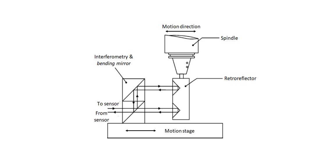
Figure 1 below shows the illustration of the reconstruction of empirical error model on a coordinate measuring machine (CMM). In this empirical model, position errors of the instrument are mapped within its measuring or working volume in term of grid.

This grid has a certain density that is a trade-off between the accuracy of the reconstructed error map and the cost to quantify the errors. For example, for a $(100\times 100 \times 100)mm$ working volume, with $1mm$ positional grid density, a total of 1000000 positional error grid points have to be determined. The error between the grid points can be estimated by interpolation (usually, linear interpolation or sometimes quadratic or non-linear interpolation to get high accuracy of interpolation).

To reduce the cost, instead of measuring 1000000 positional errors, only errors on each single axis is measured and with the kinematic error of the instrument, all other error points can be estimated. This is an example of hybrid analytical and empirical approaches.

Figure 1: Empirical error model reconstruction on an instrument based on positional grid within its measurement or working volume. (right) the measurement of positional error per each single axis motion. From this measurement, a 3D positional grid will be reconstructed and error in between the grid points will be estimated by interpolation.

The advantage of using empirical error model is that the error map obtained is representing the error in real condition of an instrument and the form of the error map is a simple mathematical form.

However, empirical error map requires many error quantifications on many locations within a measuring or working volume of an instrument or machine tools. Hence, if a high-density grid error map will be built by using an empirical approach, a long calibration time, and hence the cost, to build the empirical error map will be very high.

Instruments and software for implementing error compensation

The role of software for error compensation is vital not only for software-based error compensation but also for hardware-based error compensation. For hardware-based error compensation, software is still needed to perform interpolations to estimate errors in between points in an error map as well as to calculate how much hardware action required to compensate an error.

However, hardware of instrument is also instrumental for error compensation implementation. This hardware is used to experimentally quantify errors to build an error map.

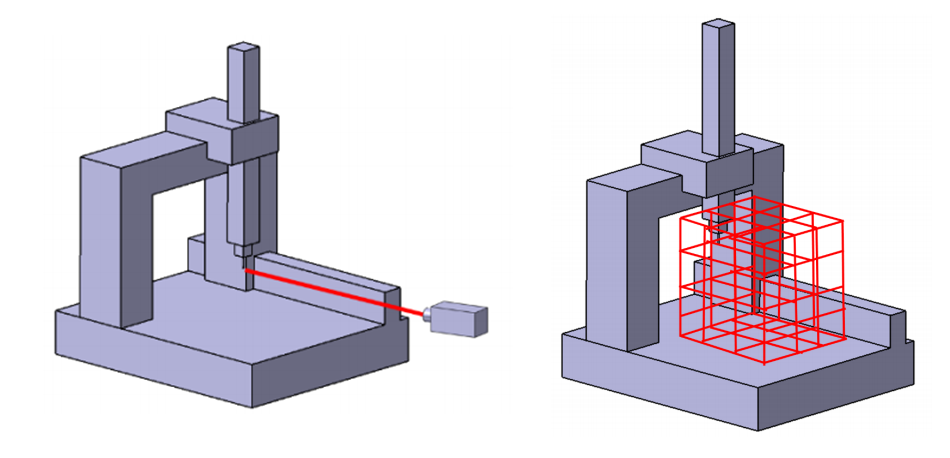
Table 1 below shows some list of instruments that are very often used to experimentally quantify errors to build an error map. Very often, errors that are experimentally determined are geometrical errors of components constructing an instrument.

Table 1: The list of instruments used to experimentally quantify errors [1].

Calibration process to quantify errors

It is known that quantifying errors on an instrument is a difficult task. There are various types and procedures to experimentally quantify each of error types [2].

One important thing to note is that instruments used to measure and quantify errors should have high accuracy and precision (significantly higher than the instrument whose errors need to be quantified) as well as traceable to the definition of meter.

Because, the essence of calibration is to create a traceability chain to the definition of meter by determining the uncertainty of the quantified errors.

In addition, in general, errors to be quantified on an instrument are usually small. Hence to be able to reliably quantify an error, the instruments used should have at least 10 times smaller error than the errors to be quantified with.

There are two main methods to perform a calibration: direct measurement method and in-direct measurement method [2].

Direct measurement method is an error measurement that can measure in axis motion direction at a time without involving the other motions from other axes.

Indirect measurement method an error measurement that involves two or more axes motion at a time.

Very common, direct measurement methods use laser interferometer systems and indirect measurement methods use calibrated artefacts, such as ball-bar in R-Test, gauge block and other calibrated artefacts.

Direct measurement method

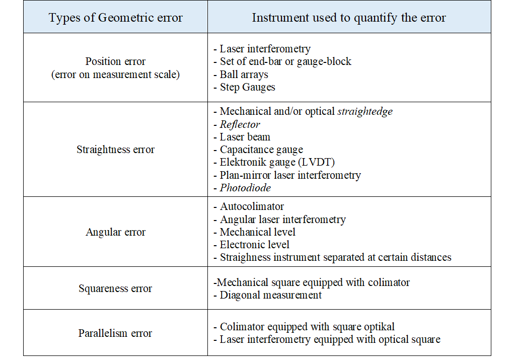
Direct error quantification or measurement for positional error, angular, straightness and perpendicularity errors very common use a laser interferometry system.

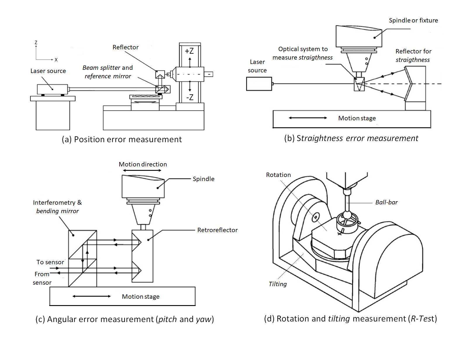
Figure 2a, 2b,2c below show the method of direct error quantifications for positional error, angular error, and axis perpendicularity error by using laser interferometer systems.

In figure 2a, the positional error of an axis by using a laser interferometer system is shown. In this measurement, an optical system consisting of a beam splitter (to divide the laser beam to a reference mirror and a retroreflector mirror to return bac the laser to an intensity sensor), and a reflector lens are used. The positional error is the difference between the commanded axis position by a control system and the axis position read by the laser interferometer.

In figure 2b, the straightness error measured by a laser interferometer is presented. On this error measurement, a different optical system (with respect to positional error measurements) is required. For this straightness measurement, the retroreflector lens is not flat, instead the lens has a “V” shape. If there is a straightness error, hence the reflected laser will not toward the middle point of the optical system.

In figure 2c, the angular error measurement is shown. The angular error that is measured is pitch and yaw error (and not roll error). In this angular error measurement, the retroreflector used is constituted by two “V” shape reflectors. On the beam splitter section, the laser is split into two parts to make two laser pathways. If there is an angular error, hence the two laser pathways will have different lengths. This different length will cause the two lasers reach an intensity sensor detector at different time so that there will be a phase difference. This phase difference is used to quantify the angular error.

One important thing to remember with regards to laser interferometer measurement is that this measurement is very sensitive to environmental variations. Small temperature, pressure and humidity variation as well as small vibration noise, will significantly and negatively affect the measurement results of the laser interferometer system.

Figure 2: Error quantification by using a laser interferometer and ball-bar. The error quantification is divided into direct and indirect measurements. Direct error quantifications: (a), (b) and (c), Indirect error quantification: (d) [2].

Indirect measurement method

Indirect measurement methods give combined measured or quantified errors obtained from more than one axis movements (multiple-axis movements).

Some examples of indirect measurement method are given in Figure 2d above for R-test and in figure 3 below for measurement of calibrated reference artefacts.

In figure 2d above, an R-test, that uses a single ball-bar with an integrated load cell, is performed to quantify or measure the error of a rotation axis. This R-test is implemented by placing one end of the ball-bar on the rotational table of the rotation axis and the other end of the ball-bar on a spindle head or something that are stable and static.

Then, the rotation axis, by which errors are to be measured, is rotated at a certain rotational speed. If there is a rotational error, the load cell on the ball bar will detect additional axial (negative or positive) stress. Since the R-test requires two-axis movements. Hence, the measured rotational errors are caused by errors from the two-axis motions.

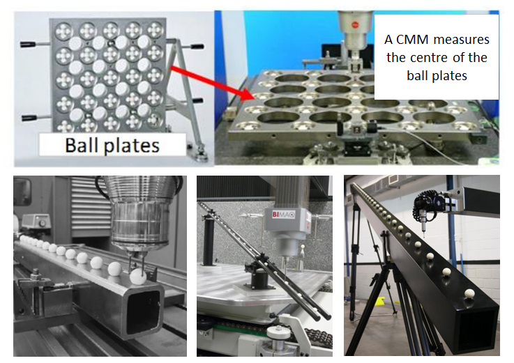
Figure 3: Other examples of indirect error quantification or measurement (other than R-test) by measuring calibrated artefacts.

From figure 3 above, indirect error measurements by measuring calibrated artefacts are shown. In figure 3, the most common calibrated artefacts are in the form of circle or sphere.

Commonly, with this method, an error is defined as the difference between a two-centre distance (of a circle or sphere) measured by an instrument of which errors are to be quantified (such as CMM) and the calibrated two-centre distance on the artefact.

To measure the circle or spheres on the artefacts, a two-axis motion is required (for example, the motion of x- and y- axes). Hence, the measured errors are the combined errors from the two axes.

One important thing to remember, the main advantage of using circle or sphere artefacts is that to measure the circle of the sphere, two-axis motions from two different symmetrical approaching directions are needed.

From these two different symmetrical approaching motions, the systematic error originated form the axis can be minimised.

Conclusion

In this post, different steps or procedures as well as different measuring instruments are required to perform error compensation on a measuring instrument or machine tools that have motion axes.

The first step for error compensation is to mathematically reconstruct the error map of an instrument, either by using analytical or empirical methods.

Different types of error to be quantified require different instruments or tools. These instruments should have at least 10 times smaller error than the error to be quantified by these instruments.

The most used instruments or tools for error quantification are laser interferometer, ball bar and circle/sphere calibrated reference artefacts.

There are two main types of error measurement: direct and indirect measurement methods. Direct measurement method only involves a single axis motion at a time. Meanwhile, indirect measurement method involves two or more axis motions at the same time.

Reference

[1] Sartori, S. and Zhang, G.X., 1995. Geometric error measurement and compensation of machines. CIRP annals, 44(2), pp.599-609.

[2] Schwenke, H., Knapp, W., Haitjema, H., Weckenmann, A., Schmitt, R. and Delbressine, F., 2008. Geometric error measurement and compensation of machines—an update. CIRP annals, 57(2), pp.660-675.

You may find some interesting items by shopping here.