GNSS signal modelling considering channel impairments and spoofing interferences
Signals of global navigation satellite system (GNSS), such as the well-known GPS and GALILEO, are significantly affected by channel impairments and signal interferences.

Signals of global navigation satellite system (GNSS), such as the well-known GPS and GALILEO, are significantly affected by channel impairments and signal interferences.
Channel impairments are any disturbances that contribute to the quality degradation of GNSS signals as well as to the addition of noise on the GNSS signals.
Examples of channel impairments are ionospheric delay, tropospheric effect, obstacles (causing signal reflection and power attenuation), non-line-of-sight (NLOS) and multipath and others.
Signal interferences are all interactions between GNSS signals and other electromagnetic waves. These interferences can be in-band or out-band as well as narrow- or wide-bandwidth.
In-band interference is where interference signals have a carrier frequency within GNSS frequency bands. Meanwhile, out-band interference is where interference signals have a carrier frequency near to the GNSS frequency and bandwidth.
In-band interference bandwidth can be, for examples, from other GNSS signals in the same frequency and band, from intentional spoofing signals or from other sources.
Hence, it is important to understand the signal behaviour due to these channel impairments and interferences. By understanding these phenomena, we can design or prepare mitigation for our GNSS receiver design.
Let us go into details!
READ MORE: Low frequency radio navigation system for use in natural disaster situations

Receiver architecture modelling for authentic GNSS signal
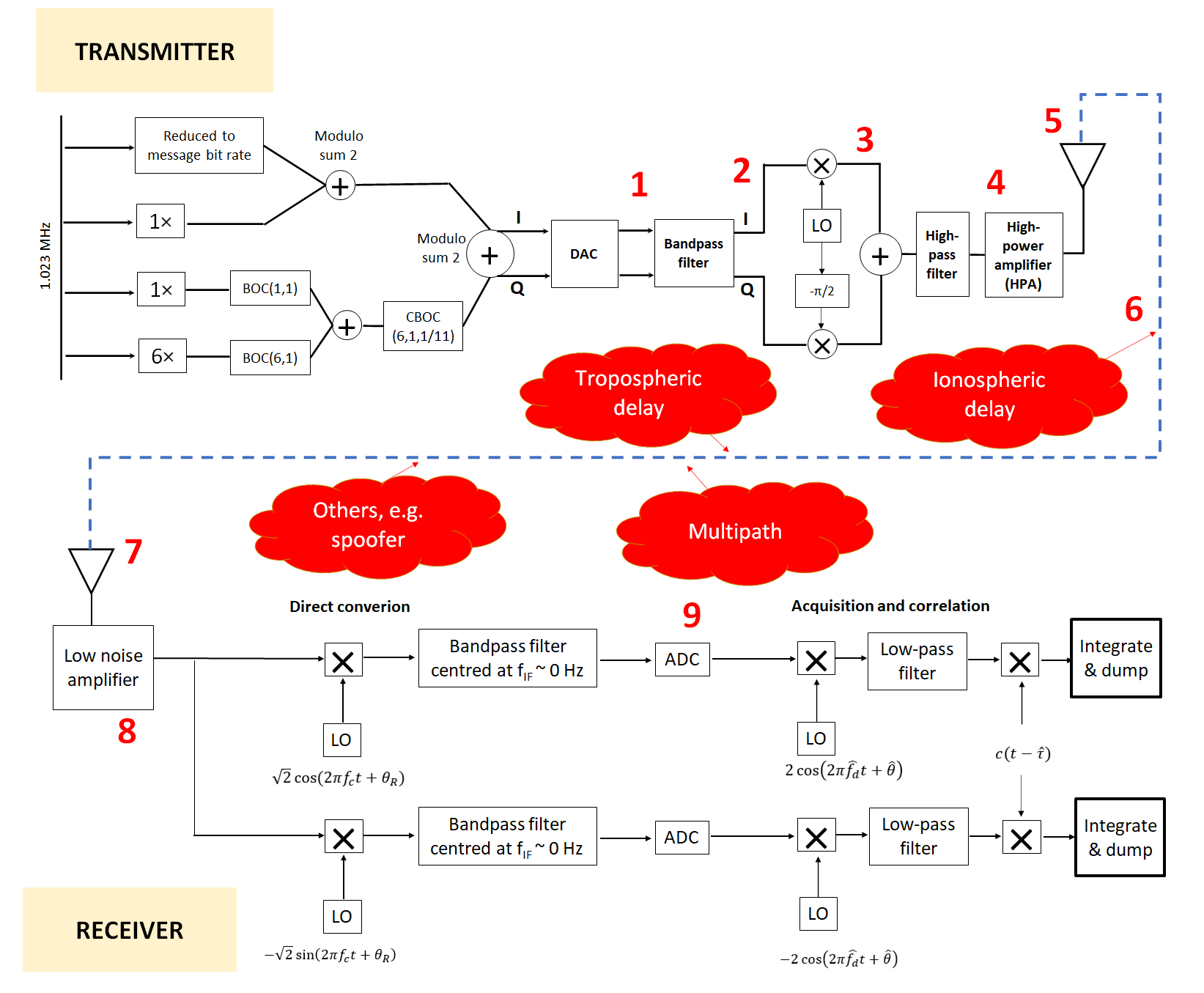
Figure 1 below shows the diagram of the mathematical model of a receiver architecture for GNSS signal. The architecture is general and is representative for various GNSS types, such as GPS and GALILEO and other GNSS signals as well.
In figure 1, the receiver architecture model is derived from [1]. However, this model is modified to represent a direct-conversion receiver.
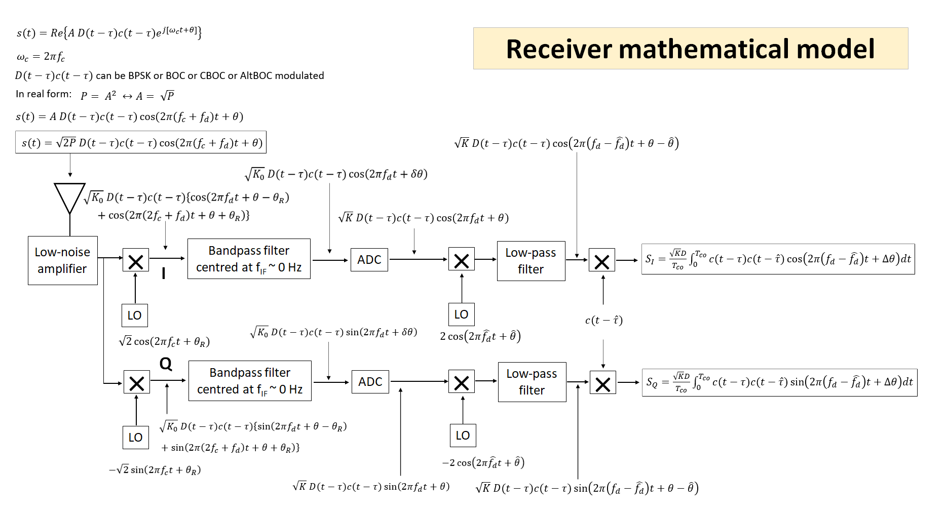
Since the receiver uses direct-conversion method (figure 1 above), the intermediate frequency (IF) at the receiver is set to 0 Hz. That is, the receiver directly down-convert a carrier frequency to baseband frequency.
The signal modelling, considering an ideal situation that is no channel impairments and no interferences, from the receiver antenna until a signal acquisition process (figure 1) as follows:
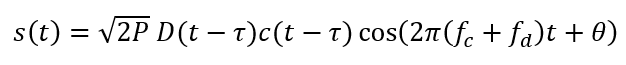
Received signal at the antennal is defined as:
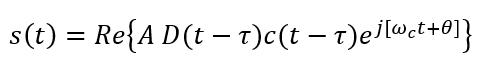
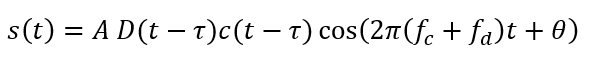
In real form, the signal becomes:
Where:
- $\omega _{c}=2\pi f_{c}$ is angular carrier frequency
- $A$ is signal amplitude
- $\tau$ is code delay during traveling from an SV to receiver, $D()$ is the data or message bit
- $c()$ is the PRN code
- $D(t-\tau)c(t-\tau)$ can be BPSK or BOC or CBOC or AltBOC modulated
(Note: the use of complex form $e^{j\theta}$ is to ease computational and mathematical representation and manipulation of the signals)
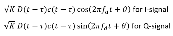
Since, $P=A^{2}/2; A=\sqrt{2P} $, hence considering only the real part (I-signal) and the signal power is distributed equally, the signal becomes:
Since $f_{IF}=0 Hz$ (direct conversion), the received signals at the RF front-end are mixed with the receiver’s local oscillator to down convert the centre frequency to be at $0 Hz$.
The local oscillators at the RF front-end to separate the I and Q phase (signal) are set to:
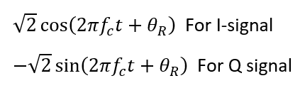
After the modulation with the local oscillator, the signals become:
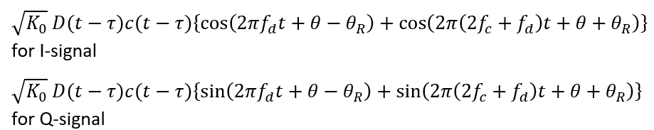
After a bandpass filter to remove high frequency components, the signals become:
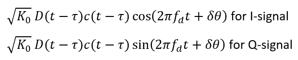
Then, after ADC conversion, the amplitude of the signals is changed, and the signal become:
After the ADC, the I and Q signals will be in digital form. These digital form signals are then digitally process following GNSS signal processing chain.
Then, the signals will go into acquisition phase to determine whether a GNSS signal is present or not. This acquisition process is to find the matched local Doppler and local PRN code combinations.
Before correlation with the local PRN code, the signal’s Doppler frequency $f_{d}$ should be removed by modulating the signal with:
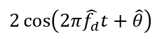
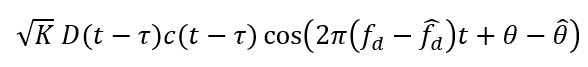
After a low-pass filter, the signal becomes:
For the Q-signal (quadrature-phase), the Doppler frequency removal is performed by modulating the signal with:
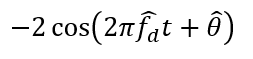
And after a low-pass filter, the signal becomes:
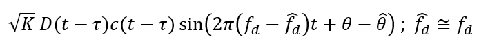
Finally, signal correlations with a local PRN code is performed as:
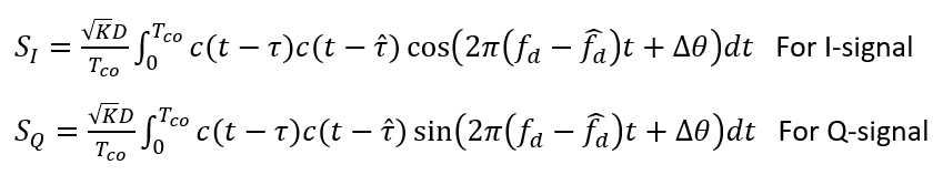
Where $T_{CO}$ is coherence integration time (in a normal open-sky GNSS signal, $T_{CO}=1 ms$).
All calculations will be performed in complex form $(e^{j\theta})$ to ease calculation .
READ MORE: Beware of reading signal-to-noise ratio (SNR) from power spectral density (PSD) plot
GNSS authentic, spoofing and spoofed signal modelling incorporating channel impairments
This modelling use GALILEO E1b signals for case study. Although using GALILEO signals, the method is also applicable for GPS signals
The model describes the E1b signals from its generation on a GALILEO satellite (SV), to a receiver and to signal tracking results.
Figure 2 below shows the E1b baseband signal where the data is on I-channel and no data on Q-channel. Q-channel is considered as a pilot signal with no data. The considered channel impairments in the model are ionospheric effect, tropospheric effect and multipath effect.
Note: all impairments are considered when signals are in analog and RF domain. That is, the effect of the channel impairments occurs from the DAC of the satellite to the ADC of the receiver (figure 2).
In figure 2, a direct-conversion receiver architecture (shown in figure 1 above) is used. the carrier frequency is 1575.42. since we consider E1b signal, the baseband rate is 1.023 MHz (following the chip rate of a PRN code used). hence the baseband bandwidths will be 2.046 MHz.
In figure 2, all received signals at a receiver are the total accumulation of authentic signals from the satellite, noises due to channel impairments, spoofing signal if any, noise from other sources (such as other GNSS signal in the spectrum bandwidth) and noise from the receiver impairments.
Transmitter signal modelling
GALILEO E1 OS signal contains two signals: E1b and E1c. The E1b signal has a primary PRN code with rate of 1.023 MHz. Meanwhile, the E1c signals has a CBOC (6,1,1/11) secondary code with rate of 6.138 MHz. The CBOC(6,1,1/11) is a combination from BOC(1,1) with rate of 1.023 MHz and BOC(6,1) with rate of 6.138 Mhz.
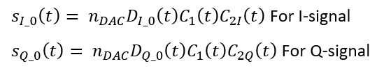
The generated nominal GALILEO E1b signals for both in-phase (I) and quadrature-phase (Q) are:
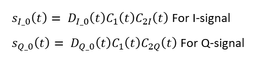
Where $C_{1}$ is the primary code and $C_{2}$ is the secondary code.
These digital nominal signals are then converted into analog signals via digital-to-analog (DAC) as shown by number 1 in figure 2). The analog signal will be affected by the power distortion or non-linearity effect from the on-board DAC hardware on the SV.
The DAC-affected signal becomes:
The analog signals after the DAC are then band-pass filtered (number 2 in figure 2) before going to a mixer for modulated with the carrier frequency at 1575.42 MHz (number 3 in figure 2). the filter at the satellite will be expected to have a good filter shape with minimal effect to the baseband signals.
After the signals are mixed with the carrier frequency (number 3 in Figure 4‑3), there will be I/Q imbalance impairments affecting the signals. Hence, the signal becomes:
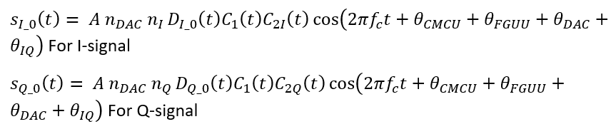
Where $\theta _{CMCU}, \theta _{FGUU}, \theta _{DAC}, \theta _{IQ}$ are the phase noise from CMCU, FGUU, DAC and IQ imbalance of the SV hardware [2,3].
Next, the signals are then amplified before being transmitted via an antenna. The signal amplification is performed by a High-Power amplifier (HPA) (number 4 in Figure 4‑3) that has a non-linearity effect [2,3]. The signals with the addition of the non-linearity of the HPA is:
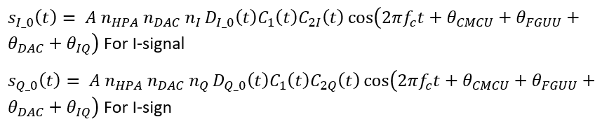
In complex form, the signals become:

Let defined:
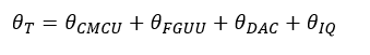
Then, the signals transmitted from the satellite (number 5 in figure 2 above) become:

After transmission, the signals will undergo channel impairments: ionospheric layer, tropospheric layer and multipath (number 6 in figure 2 above). The Ionospheric layer, tropospheric layer and multipath effect will add delay on the code phase as well as adding noises on the phase of the signals.
Hence, the signal with ionospheric effect is:

The model of the signal considering tropospheric effect is:
And, the signals with multipath effect (both Rician LOS and Rayleigh NLOS fading) is:
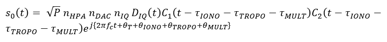
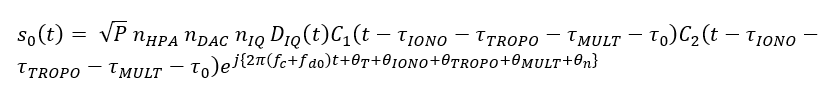
Finally, the received signals at a receiver become:

Where:
- $\theta _{n}$ is phase random noise due to other effects, such as other signals mixed with the desired signal captured withing the receiver bandwidth and other phenomena
- $f_{d0}$ is the Doppler frequency due to relative motion between the satellite and the receiver.
Receiver signal modelling
Before going through the signal modelling at the receiver, the model for received authentic signal, spoofing signal and spoofed signal are as follows:
1. Received authentic signal
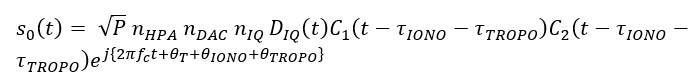
The model for the received authentic signal $s_{0}(t)$ is:
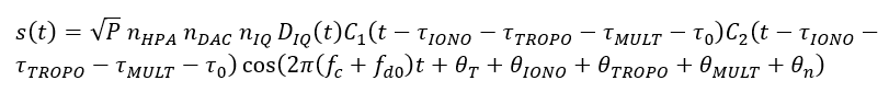
The real form:
2. Simple spoofing signal
The model for a spoofing $s_{s}(t)$ in real form is:

Note that this spoofing signal will have properties as follow:
- Different data or message bit with the authentic signal $D_{S_IQ} \neq D_{IQ}$
- The same PRN code and the secondary code with the authentic signal $C_{S_1}=C_{1}$ and $C_{S_2}=C_{2}$
- Different code delay $\tau _{S} \neq \tau _{0}$and different Doppler frequency $f_{d0}=f_{ds}$
3. Spoofed signals
The spoofed signal $S_{T}(t)$ is the addition between the authentic signal $S_{0}(t)$ and spoofing signal (spoofer) $S_{S}(t)$ as well as additional random noise $n(t)$. $S_{T}(t)$ is modelled as:
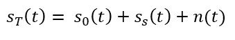
$n(t)$ represents other noises, including other PRN signals, that are not specifically considered in the model.
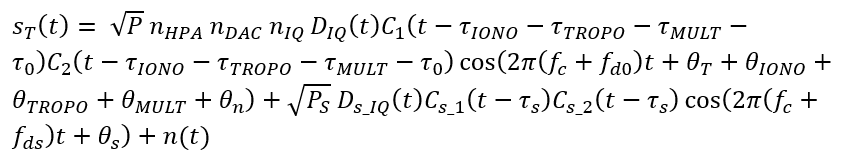
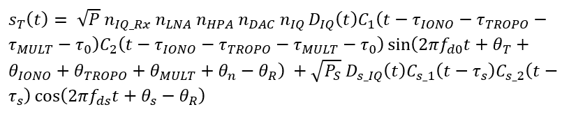
By inserting the $S_{0}(t)$ and $S_{S}(t)$ equations, hence, the real form of the model of the spoofed signal is:
Spoofed signal (authentic + spoofing signals) processed at the receiver
The receiver hardware impairments considered are receiver low-noise amplifier (LNA) non-linearity effect $n_{LNA}$, I/Q imbalance $n_{IQ_Rx}$, ADC distortion $n_{ADC}$ and the phase noise due to I/Q imbalance $\theta _{R}$.
Several conditions are considered in this modelling as follows:
- $\tau _{0} \neq \tau _{s}$; the code delay between the authentic and spoofer signals is different.
- $f_{d0} \neq f_{ds}$; the Doppler frequency between the authentic and spoofer signals is different.
- $\theta _{0} \neq \theta _{s}$; the carrier phase between the authentic and spoofer signals is different.
- $P_{0} \approx P_{s} \approx P$; the signal power between the authentic and spoofer signals is similar.
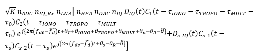
The received spoofed (containing mixing of authentic and spoofing) signals are direct converted as follow.
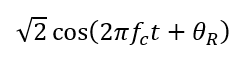
For the I-signal (in-phase), the down-conversion is by mixing with (and then bandpass filter):
The I-signal becomes:
Similarly for the Q-signal (in-phase), the frequency down conversion is performed by modulating signal the down-conversion is by mixing with (and then bandpass filter):
The Q-signal becomes:
The down converted IQ signals will have additional signal impairments due to the filtering effect.
Note that the effect of the satellite filter is negligible compared to the receiver filter due to the satellite has a much better filtering quality than a receiver.
After the filtering process, additional impairments affect the signal, that are non-linearity of the low-noise amplifier (number 7 and 8 on figure 2) and the I/Q imbalance from the local oscillator of the receiver that cause signal distortion $n_{IQ_Rx}$ and phase noise $\theta _{R}$
The next stage is converting the analog I/Q signal into digital I/Q signal via the receiver’s ADC. This ADC conversion will add another impairment (number 9 on figure 2).
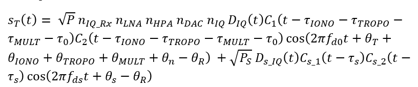
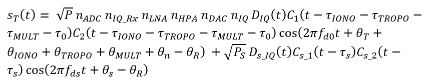
The digital form of the I-signal is:
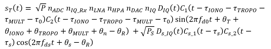
And for the Q-signal is:
Note that at this stage, the signal is already in digital form so that there are no hardware impairments on the next stage due to all processes are performed digitally (numerically).
The next step is to numerically remove the Doppler frequency before a signal correlation with local PRN code is performed.
To remove the Doppler frequency on the I-signal, the signal should be multiplied by:
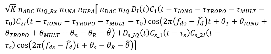
Hence, the I-signal after Doppler frequency removal is:
Similarly, to remove the Doppler frequency on the Q-signal, the signal should be multiplied by:
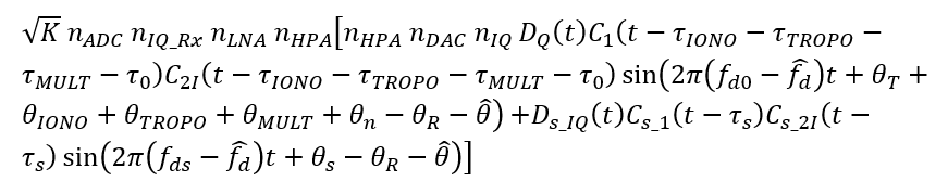
Hence, the Q-signal after Doppler frequency removal is:
For compactness, the I/Q signal is presented in a single equation in complex form as:
From this stage, signal acquisition and tracking are numerically performed.
After acquisition, assuming the receiver acquired the spoofer PRN or satellite, the estimated code delay and Doppler frequency are very close to the spoofer code delay and Doppler frequency.
Hence, the signal model becomes (in complex form):
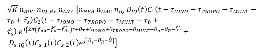
From the equation above above, the code delay and Doppler frequency at the spoofer signal part have been removed. However, the code delay and Doppler on the authentic signal part still remain.
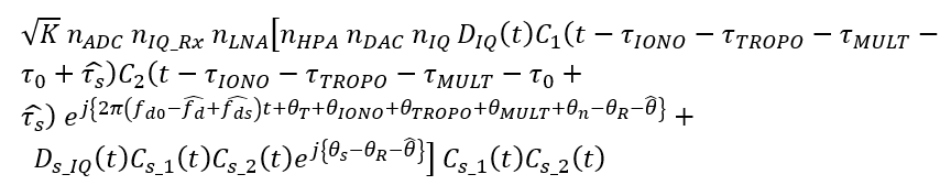
The next step is signal tracking process.
In signal tracking, the signals are correlated with the prompt code $C_{S_1}$ and $C_{S_2}$ of the spoofing signal (spoofer).
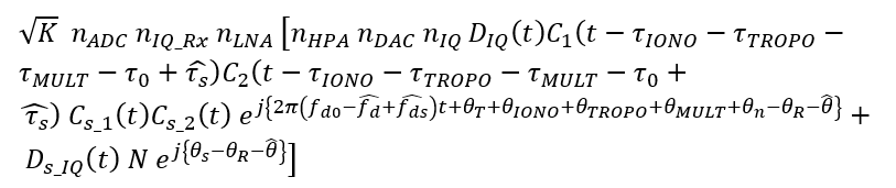
The tracked signal model (in complex form) is:
Since, $C_{S_1} C_{S_2} \times C_{S_1} C_{S_2}$ is the prompt correlation of the PRN code, the value will be a constant N and its value is number of the PRN rate. Hence, the model of the tracked spoofed signal is:
The equation above can be shortened by substituting:
M is a small value due to un-matched correlation between the PRN of the signal and the local PRN at the receiver. Hence, the shortened version of the tracked signal is:

Where:

Note that if:

There will be distortion on the correlation peak during signal acquisition. In addition, $\theta _{R}$ is slow varying because of the clock stability.
Note that the value of:
is expected to be small.
READ MORE: GNSS spoofing: a fatal attack on GNSS system that is difficult to detect
GNSS signal simulation: authentic and spoofed signals
Based on the final equation above, signal simulations are performed. The simulations are applied to the tracked IQ signals at the receiver after post-correlation.
The presentation of the simulation results is by using the constellation plot of the tracked IQ signals.
The assumptions and parameters used by the signal simulation are as follow:
- The signal simulation is assumed after correlation stage (tracking), where the noise is very small compared to the baseband signal (due to prompt correlation) and the Doppler frequency has been removed from the signals
- The noise from code and carrier tracking are not considered.
- The simulation is performed for 1 s duration of signal sampled at 25 MHz.
- All hardware impairments at the transmitter and receiver are obtained from the data sheet of a high-grade (simulate a satellite) and low grade SDR (simulate a receiver).
Figure 3a below shows the simulation of authentic signal in nominal condition without any impairments, with transmitter impairments only and with both transmitter and channel impairments.
The I/Q imbalance impairments from the receiver hardware contribute to the shifted of the I/Q signal from its nominal constellation.
As can be seen in figure 3a, the channel impairments cause a significant noise on the signals, especially from Ionospheric effect.
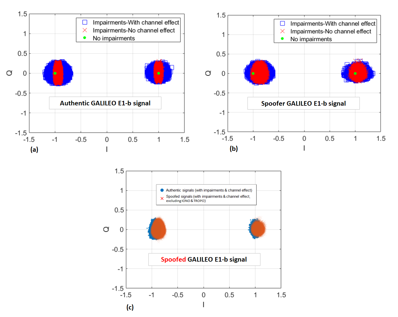
Figure 3b above shows the simulation of spoofer signal. Similarly, the I/Q signal shifting is due to I/Q imbalance and is slightly larger compared to the simulated authentic signals.
It is worth to observe that in term of signal noise (spread), by inspection, the spoofer signal has larger spread than the authentic signal. The reason is that the hardware quality generating the spoofing signal is far below the hardware quality of satellites that transmit authentic signals.
Figure 3c above shows the simulation of authentic signal and spoofed (authentic + spoofing) signal considering both hardware and channel impairments.
However, for the spoofed signal, due to the spoofing signals are from inside earth (not space), only Tropospheric and multipath effect are considered for the channel impairments. The spoofing signal will not pass the Ionospheric layer.
From the simulation results, some difference between authentic and spoofed signals can be observed, that are, for example, the shape of the signal spread and the orientation of the signal spread. These difference can be exploited, for example by machine learning methods, for spoofing detection in GNSS signals.
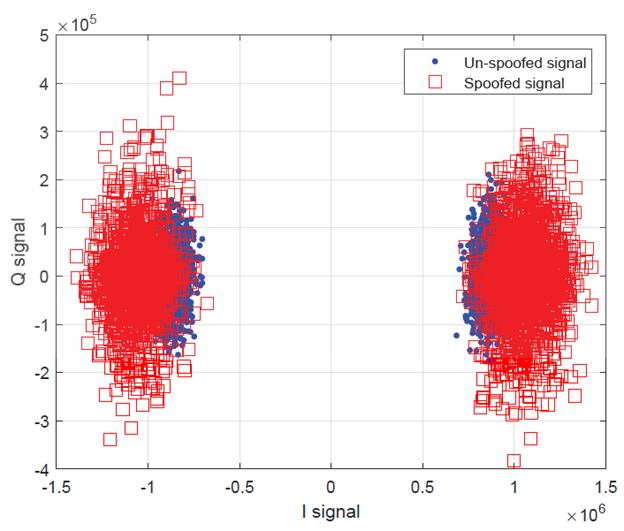
For validation of the signal modelling, figure 4 above shows the constellation plot of the tracked IQ signals of GPS L1 C/A between authentic and spoofed signals.
The authentic and spoofed signals, shown in figure 4, are produced by a high-end commercial GNSS signal simulator.
The signals statistical property and distribution shape, shown in figure 4, have a good similarity with the signals shown in figure 3c above.
One of the contributing factors between the signal generations, shown in figure 3c and figure 4, is that the hardware impairment and channel impairment values used for the simulations are different.
Conclusion
GNSS signals received by a receiver on earth are very weak because the signals are transmitted from the space.
In addition, due to long travel paths of the signals, channel impairments and signal interferences, experienced by the GNSS signals, will degrade the quality of the received GNSS signals.
This post presents and discusses GNSS receiver architecture and signals considering channel impairments and interferences.
By understanding the signal models, we can have a better understanding of GNSS signal, transmitted form a satellite in space to a receiver on earth, evolution during travelling, we can use the models to improve a GNSS receiver design and we can mitigate interferences on GNSS signals.
References
[2] Rebeyrol, E., Macabiau, C., Julien, O., Ries, L., Issler, J-L., Bousquet, M., Boucheret, M-L., "Signal Distortions at GNSS Payload Level," Proceedings of the 19th International Technical Meeting of the Satellite Division of The Institute of Navigation (ION GNSS 2006), Fort Worth, TX, September 2006, pp. 1595-1605.
[3] Benedicto, J., Dinwiddy, S.E., Gatti, G., Lucas, R. and Lugert, M., 2000. GALILEO: satellite system design and technology developments,” European Space Agency.
You may find some interesting items by shopping here.