Metrology

Mathematical geometrical fitting: Direct least-square fitting of circle geometry (with tutorial and code)

Circle is a non-linear geometry that has a non-linear mathematical model. In this post, a closed-form and deterministic method to fit a circle from points (e.g., obtained from a measurement) by using direct least-square (DLS) estimation method is presented.

Wahyudin Syam

Aug 18, 2023 • 6 min read

A DLS estimation approach can be performed by constructing “the normal equation” derived from the mathematical equation of the circle model.

The advantages of using a DLS estimation to fit a circle or other geometries are fast and deterministic.

Since the DLS method is a closed mathematical form, hence a direct computation can be performed very fast by a common computer. In addition, since random initial point generations, that are required by iterative methods, and optimisation parameters are not required, the algorithm becomes deterministic.

Hence, there is a question on why we need the complex iteration optimisation methods (such as LM algorithm) to fit a circle instead of just using this DLS approach?

The answer is that the DLS method has some fundamental drawbacks that cause the complex iterative non-linear optimisation methods are still relevant to use.

Some of the drawbacks are as follows. DLS methods only give one solution (that may or may not be optimal) and the given solution can be bias, especially for data points that do not describe or represent the geometry entirely (only represent the geometry partially, such as less than half of a circle geometry).

Additionally, in an “ill-conditioned” data points, the DLS method cannot give a single solution due to the Jacobian matrix (constructed from measured points) is singular so that the matrix cannot be inversed. A pseudo-inverse method can be used to estimate the inverse of singular Jacobian matrix, but this method will significantly deteriorate the fitting results.

Finally, sometimes, the normal equation of a geometrical model cannot be derived. And hence, DLS methods cannot be applied.

Let us go into the derivation and code implementation!

Numerical Python: Scientific Computing and Data Science Applications - A book Leverage the numerical and mathematical modules in Python and its standard library

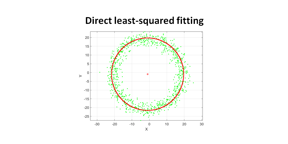
Direct least-squared fitting of circle

Direct least-squared fitting is basically a closed form parameter estimation method that involves calculating, squaring and inverting a Jacobian matrix derived from a constructed normal equation.

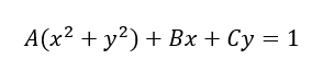
The first step of DLS method is to build the mathematical model of a circle (or other geometrical forms) and identify the fundamental parameters that define the geometry.

For circle, its geometrical equation is:

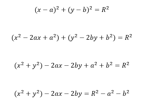
Multiplying both sides of the equation by:

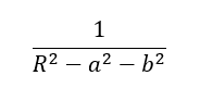
We get:

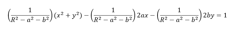
By substituting:

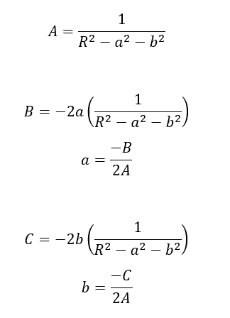
We get:

$A,B,C$ are the parameters to solve via the direct least-square (DLS) fitting method. Since there are three parameters, we need at least four points (to form four equations) to be able to perform a least-squared estimation (having an “averaging effect”).

After solving for $A,B,C$, we can get the circle centre and radius parameter $a,b,R$ from the obtained $A,B,C$ values.

Numerical Python: Scientific Computing and Data Science Applications - A book Leverage the numerical and mathematical modules in Python and its standard library

Solving the parameters of circle equation with Direct least-squared estimation

To perform a DLS estimation, we need to arrange the equation of:

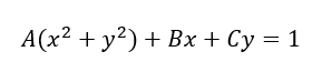
Into matrix forms.

The matrix form is:

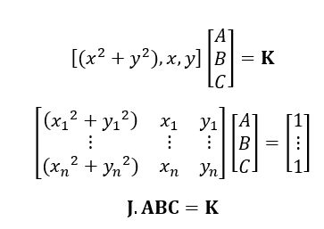
Where the J matrix is called a Jacobian matrix. The equation above is commonly called as “Normal equation”.

We multiply both side of the equation by J^T to square the matrix J:

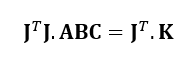
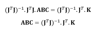
To solve for $A,B,C$, multiply both sides of the equation by (J^TJ)^-1 as follows:

Obtaining the circle parameter $a,b,R$ from the direct least-squared estimated $A,B,C$

After getting $A,B,C$ from the DLS fitting, we then can get the circle parameter values $a,b,R$.

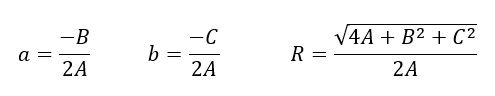
First we will find the circle centre $a,b$ as follows.

Since $a,b$ are:

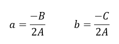
Then, $R$ can be calculated as:

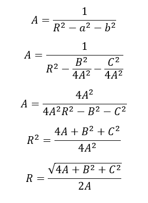
Finally, the circle parameters $a,b,R$ are calculated as:

MATLAB code for direct least-squared circle fitting

The implementation of the DLS method for circle fitting into MATLAB or any programming languages is straightforward.

The MATLAB implementation of the direct least-squared fitting of circle is as follows:

[n_row,n_col]=size(Mraw);
J=zeros(n_row,3);
M_ABC=zeros(n_row,3);
 
XX=Mraw(:,1);
YY=Mraw(:,2);
 
for ii=1:n_row
    x=XX(ii);
    y=YY(ii);
    K(ii)=1;
    J(ii,1)=x*x + y*y;
    J(ii,2)=x;
    J(ii,3)=y;
end
 
K=K';
JT=J';
JTJ = JT*J;
InvJTJ=inv(JTJ);
 
M_ABC= InvJTJ*JT*K;
A=M_ABC(1);
B=M_ABC(2);
C=M_ABC(3);
xCenterEstimated=-B/(2*A);
yCenterEstimated=-C/(2*A);
rEstimated=sqrt(4*A + B*B + C*C)/(2*A);

The MATLAB complete implementation from circle point generation, direct least-square fitting until circle plotting is as follows:

clc;
close all;
clear all;
 
%POINT GENERATION
 
%definition of center and radius
x1=15;
y1=15;
r= 20;
 
nGrid=1000;
 
%Plot the circle
theta=linspace(0,2*pi,nGrid);
[x y]=pol2cart(theta,r);
 
index=1;
for i=1:nGrid
   e1=-1+2*randn;
   e2=-1+2*randn;       
   x(index)=x(index)+e1;
   y(index)=y(index)+e2;            
   Mraw(index,1)=x(index);
   Mraw(index,2)=y(index);   
   Mraw(index,3)=1; %for homogenous coordinate
   index=index+1;    
end
 
% Direct least-squared fitting---------------------------------------------
[n_row,n_col]=size(Mraw);
J=zeros(n_row,3);
M_ABC=zeros(n_row,3);
 
XX=Mraw(:,1);
YY=Mraw(:,2);
 
for ii=1:n_row
    x=XX(ii);
    y=YY(ii);
    K(ii)=1;
    J(ii,1)=x*x + y*y;
    J(ii,2)=x;
    J(ii,3)=y;
end
 
K=K';
JT=J';
JTJ = JT*J;
InvJTJ=inv(JTJ);
 
M_ABC= InvJTJ*JT*K;
A=M_ABC(1);
B=M_ABC(2);
C=M_ABC(3);
xCenterEstimated=-B/(2*A);
yCenterEstimated=-C/(2*A);
rEstimated=sqrt(4*A + B*B + C*C)/(2*A);
 
%--------------------------------------------------------------------   
 
%Preparing data for the fitted/estimated sphere
theta=linspace(0,2*pi,nGrid);
index=1;
 
R=repmat(rEstimated,nGrid,1);
[xEstimated yEstimated]=pol2cart(theta,R');
MestimatedPoints=[xEstimated' yEstimated' repmat(1,nGrid,1)];
T=[1 0  xCenterEstimated; 0 1  yCenterEstimated; 0 0 1];
MestimatedPoints=T*MestimatedPoints';
MestimatedPoints=MestimatedPoints';
 
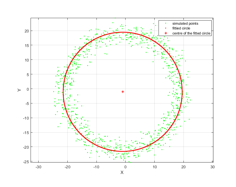
%PLOTTING
%1. Generated Points
figure(1);
plot(Mraw(:,1),Mraw(:,2),'g.');
grid on; hold on; axis equal;
 
%2. Fitted Points of the circle
plot(MestimatedPoints(:,1),MestimatedPoints(:,2),'r.');
grid on; hold on;axis equal;
plot(xCenterEstimated,yCenterEstimated,'r*');
hold on;
xlabel('X');
ylabel('Y');
legend('simulated points', 'fittied circle', 'centre of the fitted circle');
axis equal;
 
%print error betwen the center and radius
centerError=sqrt((xCenterEstimated-x1)^2+(yCenterEstimated-y1)^2);
radiusError=abs(r-rEstimated);
fprintf('center error= %f\n',centerError);
fprintf('radius error= %f\n', radiusError);

Figure 1: The simulated points and the fitted circle by using the DLS estimation.

Conclusion

In this post, we have discussed fitting a circle geometry from a point cloud by using a direct least squared (DLS) estimation method instead of an iterative non-linear optimisation method.

The advantages of the DLS method over iterative non-linear optimisations are fast (due to a direct mathematical calculation) and deterministic (it does not require random initialisation and iterative algorithm parameter settings).

However, there are some fundamental drawbacks on the DLS method that causes the iterative optimisation methods are still relevant to use. The drawbacks are the DLS method only gives one type of solution (that may or may not be optimal), produces bias (especially when the data points do not cover the entire circle or other geometry to fit) and can produce no solutions at all in “ill conditions” situation.

You may find some interesting items by shopping here.