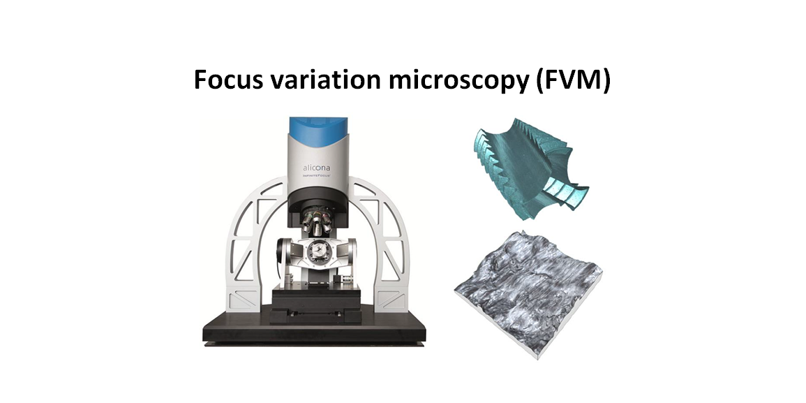
Optical measuring instrument: Focus variation microscopy (FVM) for coordinate and surface texture measurements
Focus variation microscopy (FVM) is an optical coordinate measuring machine (CMM) that is able to measure both micro-scale part geometry and areal surface texture. An FVM machine can have an up to 5-axis motion system.
Focus variation microscopy (FVM) is an optical coordinate measuring machine (CMM) that is able to measure both micro-scale part geometry and areal surface texture. An FVM machine can have an up to 5-axis motion system.
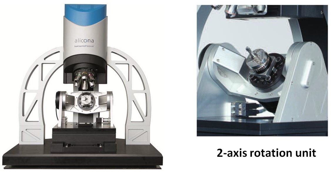
Figure 1 below shows an example of 5-axis FVM from Alicona “infinite focus G5”. The 5-axis motion is achieved by 3-axis linear motion and 2-axis rotational and tilting motion.
The FVM instrument shown in figure 1 does not use an air table for high-frequency vibration isolation. Hence, the instrument does not require a supplied compressed air for operation. Instead, a passive vibration isolation, by using a flexural component, is used on the measurement table of the instrument.
On the FVM instrument shown above, there are three types of illumination system: axial light, ring-light and polarised-light.
Axial-light is the most common type of illumination that passes through the axis of the objective lens. This type of illumination is used for common or standard surfaces that are relatively flat and not reflective.
Ring-light is the type of illumination that is off-axis of the objective lens. This type of illumination is suitable for surface with high degree of slope angle.
Polarised-light is the type of illumination with a specific filter. This filter is useful for the measurement of very high reflective surfaces. With this polarised filter, highly reflective light from a shiny surface can be reduced so that the reflective light does not saturate the 2D imaging sensor.
READ MORE: Optical measuring instrument: Point auto-focus (PAI) for coordinate and surface texture measurements
- Focus variation microscopy: performance and uncertainty evaluation- Dimensional and form measurements with optical CMMs
The working principle of focus variation microscopy (FVM)
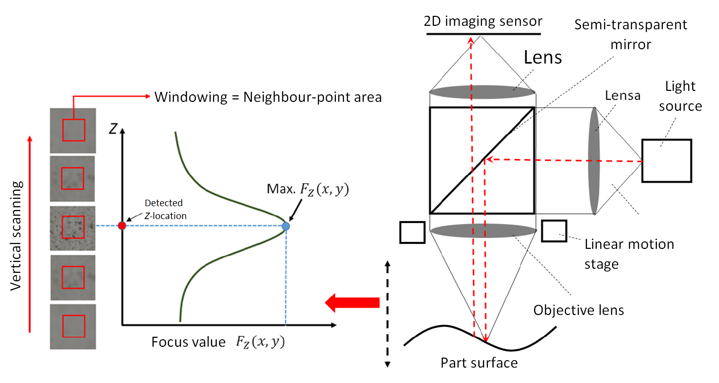
The working principle of FVM is shown in figure 2 below. FVM vertically scans the area of the surface of a part, with a pre-determined vertical resolution, and captures a sequence of 2D image on each vertical position [1,2].
From this collected sequence of 2D images of the surface during scanning, the focus value of each pixel on each 2D image is calculated. The height of each pixel location on the images is determined as the vertical location where the calculated focus (contrast) value is the largest.
The focus value $F_{Z}(X,Y)$ is calculated as:
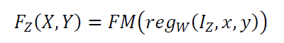
Where $I_{Z}$ is the pixel intensity value at a certain $z$-location and is associated on a specific lateral (pixel) location $(x,y)$ on the 2D imaging sensor on the FVM. $FM$ is a measured of focus that represents the contrast of a lateral $(x,y)$ location with respect to a certain neighbour points.
Figure 2 (left) above shows the process to determine the focus value for each pixel location to estimate the height of the surface at this lateral location. From this figure 2 left, if the $z$-location (height) of the vertical location is at the height of the measured surface, hence the pixel on that height will be sharp, that is, the focus value $F_{Z}(x,y)$ is the largest compared to other values at different height or $z$-location.
The optical configuration of FVM is shown in figure 2 (right) above. In principle, the optical configuration is similar or even the same as other normal microscope configurations. However, the microscope used by FVM is linearly moved by a motor to vertically scan the surface through the surface focus position.
There are several method to calculate focus value $F_{Z}(x,y)$ on a pixel. These several common methods are [1]:
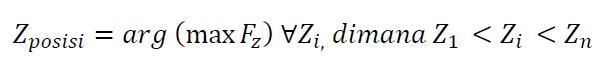
1. Maximum point method
The maximum point method is the simplest method to calculate a focus value. This method is the fastest to estimate the $z$-location or height of a pixel.
However, this method has the lowest accuracy compared to other focus value determination method.
The maximum point method is formulated as:
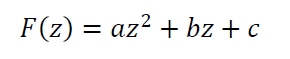
2. Polynomial curve fitting method
Polynomial curve fitting method is the method to determine the $z$-location for a lateral pixel position by fitting a quadratic curve or polynomial to the calculated focus value for each height on each pixel lateral location.
From the fitting, the height corresponding to the largest focus value can be determined. The polynomial curve fitting is formulated as:
From the above equation, the $z$-location or height for each pixel can be calculated as:
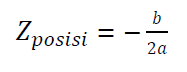
The quadratic fitting method to fit $F(z)$ is determine by using least-square method as follow:
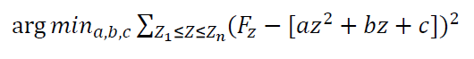
Where $a,b,c$ the parameters that need to be estimated by using the polynomial least-square fitting.
3. Point spread function fitting method
The point spread function fitting method is the method that has the highest accuracy to estimate the z-location or height of each pixel representing the lateral location of a surface. However, this method requires high computational effort.
The fitting process of this method use the point spread function of the microscope system used by an FVM instrument.
READ MORE: Optical coordinate measuring machine (Optical-CMM): Two fundamental limitations
- Focus variation microscopy: performance and uncertainty evaluation- Dimensional and form measurements with optical CMMs
Applications of focus variation microscopy (FVM)
The application of FVM instrument for micro-scale areal geometrical and surface texture measurement are wide: from dimensional, geometrical to surface texture or topography.
FVM instrument is very suitable to measure a surface having roughness $R_{a}>20nm$. However, special optics and algorithms can puh the FVM measurement capability beyond this roughness limitation.
Common surfaces that are very suitable to be measured by FVM are surfaces from machining processes, such as milling, turning, drilling and other manufacturing processes such as casting and injection moulding.
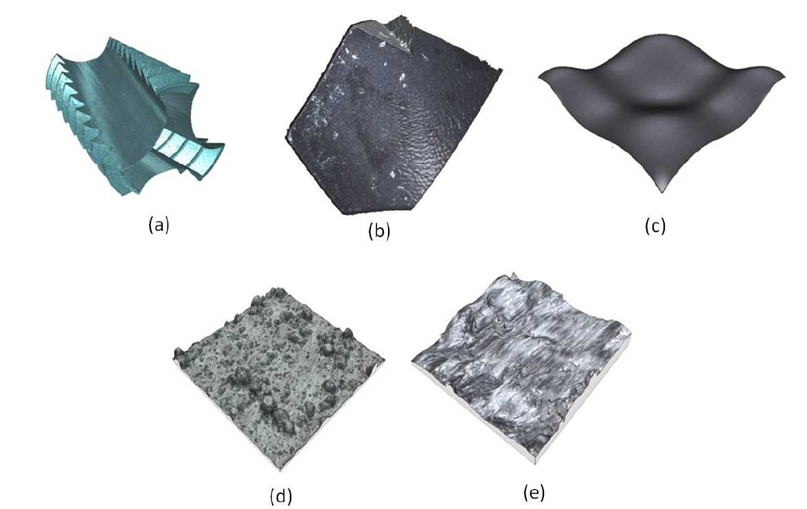
Figure 3 below presents examples of measurement results obtained by using a FVM instrument. In figure 3 (a,b,c), the example of 3D geometrical measurements of a drilling tool, the flank of a milling tool and machined free-form surface are shown. The drilling tool measurement is obtained by using the 2-axis rotation unit of the mentioned FVM.
In figure 3 (d,e), the measurement of surface texture of spray-coated surface and additively manufactured metal surface are shown.
The advantage and disadvantages of focus variation microscopy (FVM)
Every measuring instrument has both advantages and disadvantages.
The advantages of FVM instrument are:
- FVM can be used for both areal geometrical and surface texture measurement at micro-scale. The Alicona G5 mentioned above has 5x objective lens with long working distance of 23 mm. This long working distance has a significant advantage to access surfaces with complex geometry without collision between the objective lens and a measured surface [2].
- FVM is commonly less sensitive to vibration noise, pressure variation and temperature variation compared to interferometry-based measuring instrument. The reason is that, FVM is purely based on image processing method instead of interferometry method.
- FVM has a relatively fast measuring process. In general, FVM measurement for a single image field (typically ranging from around (0.1 x 0.1) mm to (5 x 5) mm, depending on the magnification of the objective lens) requires less than or few minutes.
- The mentioned FVM above has the 2-axis rotational and tilting axis for full 3D measurement of rotational parts or cylindrical as well as spherical surfaces, such as cutting tools.
- The mentioned FVM above has three optional illumination sources for various types of surfaces with different slope and reflectivity properties. The three types of illumination are axial light, ring light and polarised light.
The disadvantages of FVM instrument are:
- FVM has difficulty to measure a very smooth and shiny surface (typically with $R_{a}<10 nm$. This difficulty is caused by FVM measurements require some degree of texture (roughness) on a measured surface to calculate the focus value for each lateral pixel location and hence determine the surface height.
- The limitation of the depth of focus of the objective lens of a FVM instrument causes different height within the range of the depth of focus will have similar focus value and hence reduces the accuracy of the estimated height or $z$-location.
- FVM has difficulty to measure a transparent surface. Because beside a transparent surface has very smooth surface, the optical microscope of the FVM cannot see the surface itself (due to transparency).
READ MORE:The history and introduction of CMM: the inseparable relation between CMM and GD&T
- Focus variation microscopy: performance and uncertainty evaluation- Dimensional and form measurements with optical CMMs
Conclusion
In this post, FVM optical measuring instrument is presented in detail. FVM has a wide range of measurement applications ranging from dimensional, geometrical to areal surface texture measurements.
The working principle of FVM is purely based on image processing instead of interferometry. This image processing method causes FVM instrument is less sensitive to vibration, temperature and pressure variation compared to other interferometry-based measuring instruments.
Finally, important advantages and disadvantages of FMV optical instrument are presented and discussed.
References
[1] Leach, R. ed., 2011. Optical measurement of surface topography (Vol. 8). Berlin Heidelberg, Germany: Springer Berlin Heidelberg.
[2] Moroni, G., Syam, W.P. and Petrò, S., 2018. A simulation method to estimate task-specific uncertainty in 3D microscopy. Measurement, 122, pp.402-416.
You may find some interesting items by shopping here.
- Focus variation microscopy: performance and uncertainty evaluation- Dimensional and form measurements with optical CMMs