Demystifying p-value in analysis of variance (ANOVA)
In analysis of variance (ANOVA), p-value is very often used to determine whether an initial hypothesis is accepted or rejected. However, many people still do not know what p-value is. In fact, there is a better parameter to use to accept to reject an initial hypothesis.
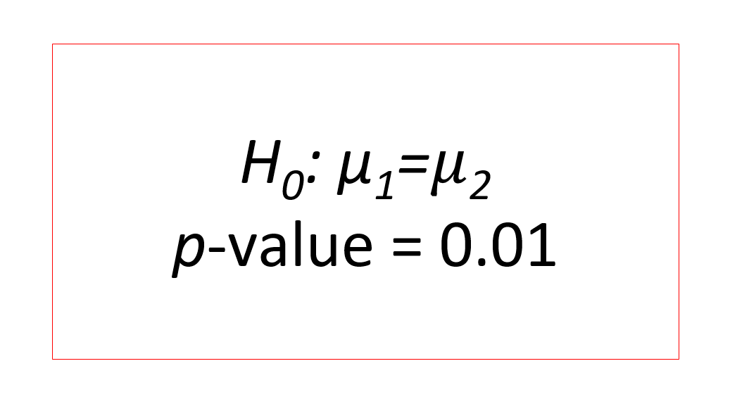
In analysis of variance (ANOVA), p-value is very often used to determine whether an initial hypothesis ($H_{0}$) is accepted or rejected. However, many people still do not know what p-value is. In fact, there is a better parameter to use to accept to reject an initial hypothesis.
In this post, we will discuss what p-value is and what quantitively a better parameter to use to accept or reject hypothesis.
Let us go into the discussion!
Analysis of variance (ANOVA): A practical introduction
ANOVA analysis was first developed by R. Fischer in 1920. The main goal of Fischer was to analyse and improve the productivity of farm crops.
ANOVA is one of the most used and common tools in statistics and data analysis. This analysis has many applications in all fields, including engineering, medicine, exact science and social science.
With ANOVA analysis, we can perform a simultaneous analysis of effects or factors, with more than two levels or treatments for each effect or factor, of an experiment or observation.
The simultaneous analysis can be done because ANOVA is the results of the generalisation of t-test analysis with two levels or treatments to test the mean equality from two types of population. Hence, the ANOVA can be used to test the mean equality for more than two types of population.
A very common example of ANOVA analysis in measurement science is to analyse, optimise and improve various types of industrial and measurement processes with gauge repeatability and reproducibility (GR&R) test.
Another example of ANOVA analysis to optimise a measurement process is to optimise the value of scanning speed parameter and number of sampled points in a geometric measurement process using coordinate measuring machine (CMM). This optimisation process is performed so that the measurement can have minimal measurement uncertainty.
In this practical introduction, the basic model of ANOVA test, that is one-way ANOVA, will be presented. This basic model of ANOVA is the basis of all others and more complex ANOVA analyses.
The basic ANOVA analysis is presented with example as follow.
Suppose, we have an experiment to optimise the heat treatment process of a material. We want to analysis one factor that affect the process that is temperature with various levels m (100 degree C, 200 degree C, 300 degree C). We want to compare these m levels to find which level gives the best treatment result. Level mcan be called as the number of treatments or levels.
On each level, experiments are repeated r times. Hence, the measurement results of the heat threated materials from the experiment are random variables.
The data observation model of one-way ANOVA analysis shown in table 1. In table 1, the data table contains $y_{ij}$ that represents the $j$-th observation at the $i$-th treatment.
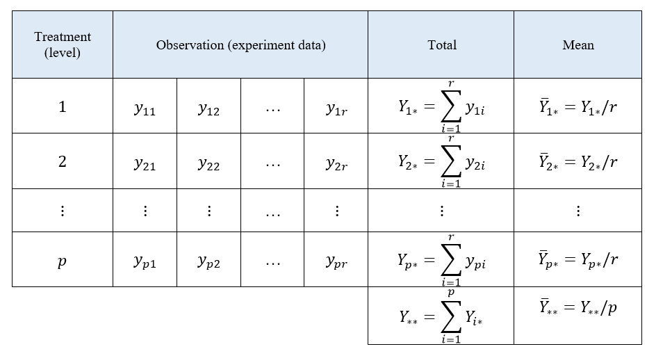
From the data structure shown in table 1 above, the data can be modelled as:
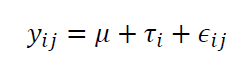
Where $i=1,2,…,p$ and $j=1,2,…,r$. $\mu$ is the mean and is constant. $\tau _{i}$ is a random variable from the $i$-th treatment or level. $\epsilon _{ij}$ is the error random variable.
The model above is assumed such that $\tau _{i} \sim N(0,\sigma _{\tau}^{2})$ and $\epsilon _{ij} \sim N(0, \sigma _{\epsilon}^{2})$.
In ANOVA analysis, there are two main types of model:
- Random-effect model
- Fixed-effect model
Random-effect model assumes that a treatment represents a random sample from a population. Hence, random-effect model has a conclusion that can be generalised to the population where the sample drawn from.
Fixed-effect model has a limited conclusion from an analysis result and the conclusion cannot be generalised to other similar treatment. Fixed-effect model has treatments or levels that are selected specifically by a person who does the experiment.
Hence, fixed-effect model (by assuming that $\tau _{i}=\tau=constant$ ) can be formulated as:
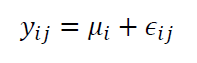
Where Where $i=1,2,…,p$ and $j=1,2,…,r$. $\mu _{i}$ is the mean and is constant and $\epsilon _{ij}$ is the error random variable. Also, $\epsilon _{ij} \sim N(0, \sigma _{\epsilon}^{2})$.
The main hypothesis from the fixed-effect model is to compare whether the mean from treatments $\mu _{i}$ is statistically equal or not equal.
Meanwhile, the main hypothesis from the random-effect model is to compare the variation of treatments whether the variation is homogenous or not.
By considering fixed-effect model, the ANOVA analysis is started by partitioning the total variation into several components that are:
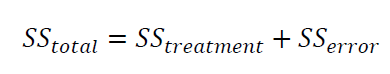
Where $SS_{total}$ is the sum-of-squared of total, $SS_{treatment}$ is the sum-of-squared of treatment and $SS_{error}$ sum-of-squared of error in all treatments.
The explanation of $SS_{total}= SS_{treatment}+ SS_{error}$ is as follow. $SS_{total}$ that is the measure of total variation in experiment data (including treatment and error) can be formulated as:
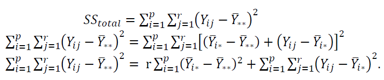
The equations above mean that the total variation from observation or experiment data, $SS_{total}$, can be partitioned into the sum-of-squared of the difference between the treatment mean and total mean plus the sum-of-squared of the difference between an observation in each treatment and the treatment mean.
The total of observations is $pr$. Where $p$ is the number of treatment or level and $r$ is the number of repetition for each treatment or level.
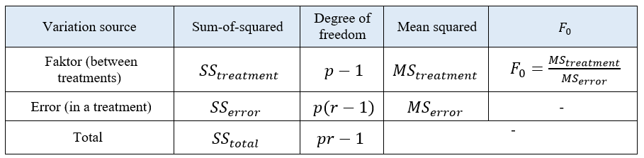
Hence, $SS_{total}$ has $pr-1$ degree of freedom, $SS_{treatment}$ has $p-1$ degree of freedom and $SS_{error}$ has $p(r-1)$ degree of freedom (because, for each repetition, the degree of freedom of the error is $r-1$).
By dividing each sum-of-squared $SS$ with its degree of freedom, we get:
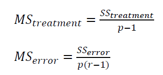
Where $MS_{treatment}$ and $MS_{error}$ are the mean-squared of treatment/level and error, respectively.
The hypothesis test of the fixed-effect model is:
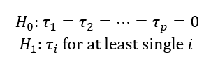
The test statistic for the hypothesis test of the fixed-effect model above is as follow:
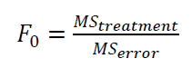
$F_{0}$ has F statistical probability distribution. If $F_{0}>F_{\alpha , p-1, pr-p}$, then $H_{0}$ is rejected and a conclusion can be said that there is a significant difference among the treatment/level mean, and otherwise.
The ANOVA table for one factor and many treatment/level fixed-effect model is shown in table 2.
Meanwhile, figure 1 shows an example of $F$ distribution. From figure 1, if $F_{0}>F_{\alpha, 4,20}$, then $H_{0}$ hypothesis will be rejected. And otherwise, if $F_{0} \leq F_{\alpha, 4,20}$, then $H_{0}$ hypothesis will be accepted.
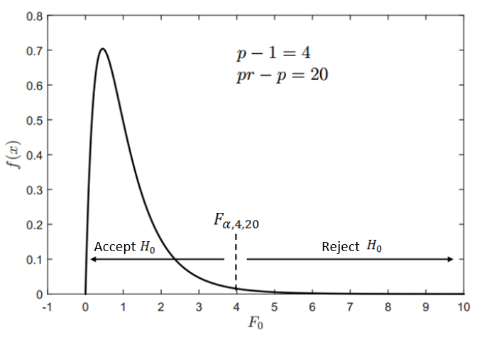
Hence, the $F_{0}$ is a better parameter to determine whether to accept or reject hypothesis $H_{0}$. Because, in ANOVA calculations and summary, $F_{0}$ values for each factor are shown. Hence we can thoroughly compare this $F_{0}$ value among each other. The $F_{0}$ that is significantly big suggests that we must reject $H_{0}$.
Demystifying p-value in ANOVA analysis
Commonly, ANOVA analysis is performed by using a commercial statistic software such as Minitab or SPSS.
For ANOVA analysis that is performed with these commercial software, very often, these commercial software will convert the $F_{0}$ value (that is the test statistic for an hypothesis test) into $p$-value.
The value of $F_{0}$ is inversely equal to $p$-value. If the $F_{0}$ value is large, then the $p$-value will be small so that we will reject $H_{0}$. And otherwise, if the $F_{0}$ value is low, then the $p$-value will be large so that we will accept $H_{0}$.
The question is, what is actually the $p$-value?
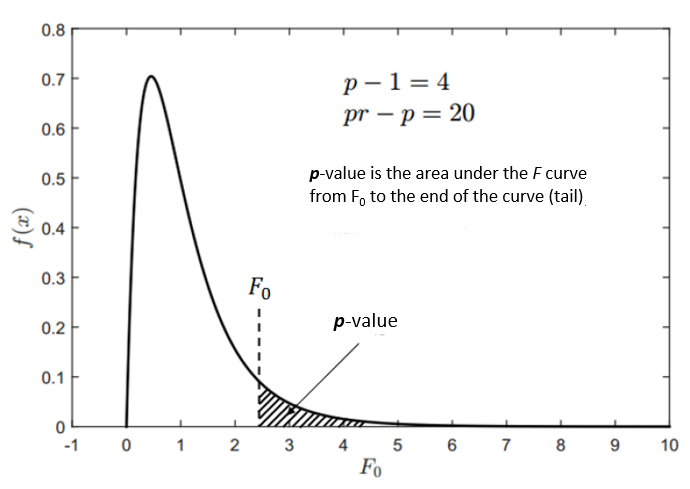
$p$-value is the area under an $F$ distribution curve from $F_{0}$ until the tail of the $F$ distribution. That is $p$-value = $P(F_{0}<X<\infty)$.
That is why, the $F_{0}$ and $p$-value have an inverse relation. Because, the larger the value of $F_{0}$, the smaller (the lower probability) the area under an $F$ distribution curve from $F_{0}$ to the tail.
Figure 2 shows the illustration of $p$-value and its relation to $F_{0}$.
ANOVA analysis with Random-effect model
For ANOVA analysis with random-effect model, aspects that are compared are the variations between treatments or levels. That is why, this model is the basic model used for Gauge R&R test.
The hypothesis test for random-effect model is:
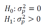
It is important to note that, for ANOVA with one factor (one-way ANOVA), the parameters of the statistical test for random-effect model is equal to fixed-effect model. However, the test statistic will be different if the ANOVA analysis has more than one factor.
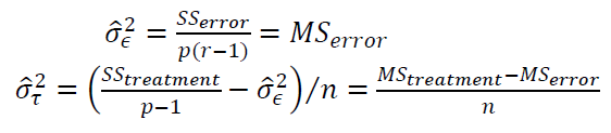
To estimate the variation for each component in the random-effect model (from the treatment, error and total), the estimation is formulated as follow:
Conclusion
In this post, we have demystified $p$-value in ANOVA analysis.
This $p$-value is always used to accept or reject hypothesis $H_{0}$ in ANOVA analysis.
However, as being explained in this post, $F_{0}$ is a better parameter to use in accepting or rejecting the hypothesis. Because, the values of $F_{0}$ are always available for each factor.
Hence, we can thoroughly compared the $F_{0}$ values for each factor. The one that is significantly big, shows that we must reject $H_{0}$.
We sell all the source files, EXE file, include and LIB files as well as documentation of ellipse fitting by using C/C++, Qt framework, Eigen and OpenCV libraries in this link.
We sell tutorials (containing PDF files, MATLAB scripts and CAD files) about 3D tolerance stack-up analysis based on statistical method (Monte-Carlo/MC Simulation).